Introduction
This analysis generates MDS plots to visualize sample groups and batch effects using the limma and edgeR packages. Following the guide “RNA-seq analysis is easy as 1-2-3 with limma, Glimma and edgeR” (Law et al. 2018), see https://pmc.ncbi.nlm.nih.gov/articles/PMC4937821/.
Setting up the data
This data was processed as follows:
- cutadapt to trim adapter sequences (but it was NOT done correctly because I used the sample barcode and not the adapter sequence).
- Hisat2 for gene-based alignment.
- RSubread featureCounts to convert to a count matrix. The alignment step showed only 3% of reads were mapped.
This is a lane-based analysis, so the lane information is still present in the count matrix. This allows us to see if there are any differences between the lanes for the same sample.
Show code
# Load required libraries for the document
library(here)
library(limma)
library(edgeR)
library(RColorBrewer)
library(ggplot2)
library(gridExtra)
library(dplyr)

# Read in count data
counts <- read.table(here("data/counts/count_matrix.txt"), header=TRUE, row.names=1, sep="\t")
colnames(counts) <- gsub("\\.\\.\\.data\\.samtools\\.|_sorted\\.bam", "", colnames(counts))

gene_info <- counts[, 1:5]
counts <- counts[, 6:ncol(counts)]
counts <- as.matrix(counts)

# Read in sample sheet
samples <- read.csv(here("data/sample_sheet_lane.csv"))
samples$group <- samples$Group
samples$Group <- NULL

# The sample sheet is already in the correct order
identical(match(samples$Name, colnames(counts)), 1:48)
Reading in count data
First we create a DGEList from the count data and the sample sheet. The count data contains a column for each lane of the experiment (48 in total). The sample sheet includes information about the mouse genotype and the batches.
The DGEList object includes counts for the numeric data, and the samples and genes data frames, which contains information about the samples and features, respectively.
Show code
# NOTE: I could have just done this using the unmodified count data
# Read in data
dge <- DGEList(
    counts,
    samples = samples,
    genes = data.frame(Length = gene_info$Length))
class(dge)
[1] "DGEList"
attr(,"package")
[1] "edgeR"Organising sample information
Show code
group <- dge$samples$group
lane <- gsub(".+_", "", dge$samples$Name)
batch <- gsub(".+_", "", dge$samples$group)
treatment <- gsub("_.+", "", dge$samples$group)

# Make sample info factors
group <- factor(group, levels=c("WT_1_B2", "WT_2_B1", "WT_3_B1",
    "SOCS3_1_B2", "SOCS3_2_B1", "SOCS3_3_B1"))
lane <- factor(lane)
batch <- factor(batch)
treatment <- factor(treatment, levels=c("WT", "SOCS3"))

# Add sample info into samples slot.
dge$samples$lane <- lane
dge$samples$batch <- batch
dge$samples$treatment <- treatment
There are 6 mice, each split across the 8 lanes.
Show code
table(group, treatment) treatment
group WT SOCS3
WT_1_B2 8 0
WT_2_B1 8 0
WT_3_B1 8 0
SOCS3_1_B2 0 8
SOCS3_2_B1 0 8
SOCS3_3_B1 0 8Show code
table(group, lane) lane
group L001 L002 L003 L004 L005 L006 L007 L008
WT_1_B2 1 1 1 1 1 1 1 1
WT_2_B1 1 1 1 1 1 1 1 1
WT_3_B1 1 1 1 1 1 1 1 1
SOCS3_1_B2 1 1 1 1 1 1 1 1
SOCS3_2_B1 1 1 1 1 1 1 1 1
SOCS3_3_B1 1 1 1 1 1 1 1 1Organising gene annotations
After mapping the sequencing reads to the genome, we have Ensembl-style identifiers.
These are used by mapping tools as they are unambiguous and highly stable.
We use the Mus.musculus package to match these IDs to gene symbols and to obtain chromosome information, for easier interpretation of the results.
Show code
# BiocManager::install("Mus.musculus")
library(Mus.musculus)
geneid <- rownames(dge)
geneid <- gsub("\\..+", "", geneid)

table(duplicated(geneid))

# We have Ensembl ID's
gene_map <- AnnotationDbi::select(Mus.musculus, keys=geneid, columns=c("SYMBOL", "TXCHROM"),
                keytype="ENSEMBL")
# Initially there are duplicate ENSEMBL id's
table(duplicated(gene_map$ENSEMBL))
# Index so the rownames are the same as the dge.
gene_map <- gene_map[match(geneid, gene_map$ENSEMBL), ]

stopifnot(identical(geneid, gene_map$ENSEMBL))

# There are thousands of duplicate symbols.
table(duplicated(gene_map$SYMBOL))
# No duplicate ENSEMBL id's now.
table(duplicated(gene_map$ENSEMBL))

# Add symbol to genes.
dge$genes$SYMBOL <- gene_map$SYMBOL
dge$genes$ENSEMBL <- rownames(dge$genes)
dge$genes$CHR <- gene_map$TXCHROM
There are some Ensembl IDs which map to the same gene symbols. For these features we will refer to the genes using both the Ensembl ID and the symbol, for example
Show code
library(scuttle)

rownames(dge) <- uniquifyFeatureNames(dge$genes$ENSEMBL, dge$genes$SYMBOL)
# Duplicate features with symbols have their ID concatenated.
# rownames(dge)[duplicated(dge$genes$SYMBOL) & !is.na(dge$genes$SYMBOL)]
# Now there are unique rownames.
table(duplicated(rownames(dge)))
Unfortunately, there is no expression using this particular Cre transcript. Hopefully something I use in the future will work better (or this becomes not necessary). Good that all the Socs genes are expressed though!
We remove features which aren’t expressed in any samples and lanes of our data.
Show code
genes_of_interest <- c("Cre", "Socs1", "Socs3", "Bcl3")In doing this we also check that this have not removed any of our genes of interest, which include Socs1, Socs3 and Bcl3. Reassuringly, these features are not removed during this step and thus have some expression in the data.
Show code
[1] TRUE FALSE FALSE FALSEShow code
# Remove features which aren't expressed in any samples.
dge <- dge[(rowSums(dge$counts) > 0), ]
Pre-processing
Filter low quality genes
Show code
# There are no genes that are expressed in no sample (48 lanes) as I already
# removed them.
table(rowSums(dge$counts == 0) == 48)
# The smallest amount of counts for a gene is 1 across the 48 samples
min(rowSums(dge$counts))

keep.exprs <- filterByExpr(dge, group=group)
dge <- dge[keep.exprs,, keep.lib.sizes=FALSE]
dim(dge)
# We have removed 20792 genes using filterByExpr.
# This function keeps genes with about 10 read counts or more in a minimum
# number of samples.
sum(keep.exprs == FALSE)
Filtering using FilterByExpr from the edgeR package removes genes with very low expression.
We retain 12179 genes for further analysis, and remove 20792 genes.
These low quality genes result in a spike near 0 in the left-hand side of the plot below.
Show code
# Figure 1: Density of the raw post filtered data

# M is the mean, L is the median
L <- mean(dge$samples$lib.size) * 1e-6
M <- median(dge$samples$lib.size) * 1e-6

lcpm.cutoff <- log2(10/M + 2/L)
library(RColorBrewer)
nsamples <- length(unique(group))
col <- brewer.pal(nsamples, "Paired")
par(mfrow=c(1,2))
plot(density(lcpm[,1]), col=col[1], lwd=2, ylim=c(0,0.26), las=2, main="", xlab="")
title(main="A. Raw data", xlab="Log-cpm")
abline(v=lcpm.cutoff, lty=3)
for (i in 2:nsamples){
  den <- density(lcpm[,i])
  lines(den$x, den$y, col=col[i], lwd=2)
}
legend("topright", as.character(unique(group)), text.col=col, bty="n")
lcpm <- edgeR::cpm(dge, log=TRUE)
plot(density(lcpm[,1]), col=col[1], lwd=2, ylim=c(0,0.26), las=2, main="", xlab="")
title(main="B. Filtered data", xlab="Log-cpm")
abline(v=lcpm.cutoff, lty=3)
for (i in 2:nsamples){
  den <- density(lcpm[,i])
  lines(den$x, den$y, col=col[i], lwd=2)
}
legend("topright", as.character(unique(group)), text.col=col, bty="n")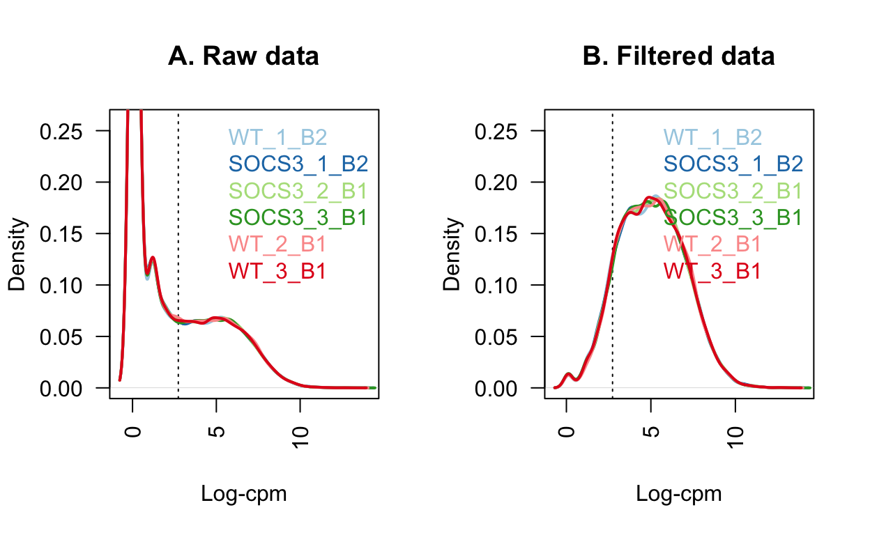
Normalisation
Visualising the data
Show code
# Set colours for this data set
group_colours <- setNames(
    ggthemes::tableau_color_pal("Tableau 10")(6),
    levels(group))

lane_colours <- setNames(
    brewer.pal(nlevels(lane), "Set2"),
    levels(lane))

batch_colours <- setNames(
    brewer.pal(8, "Dark2")[3:4],
    levels(batch))

treatment_colours <- setNames(
    brewer.pal(8, "Dark2")[1:2],
    levels(treatment))
Show code
# MDS plots
par(mfrow=c(2,2))
plotMDS(lcpm, labels=group, col=group_colours[group])
title(main="A. Sample groups")

plotMDS(lcpm, labels=treatment, col=treatment_colours[treatment])
title(main="B. Treatment")

plotMDS(lcpm, labels=batch, col=batch_colours[batch])
title(main="C. Batch")

plotMDS(lcpm, labels=lane, col=lane_colours[lane])
title(main="D. Sequencing lanes")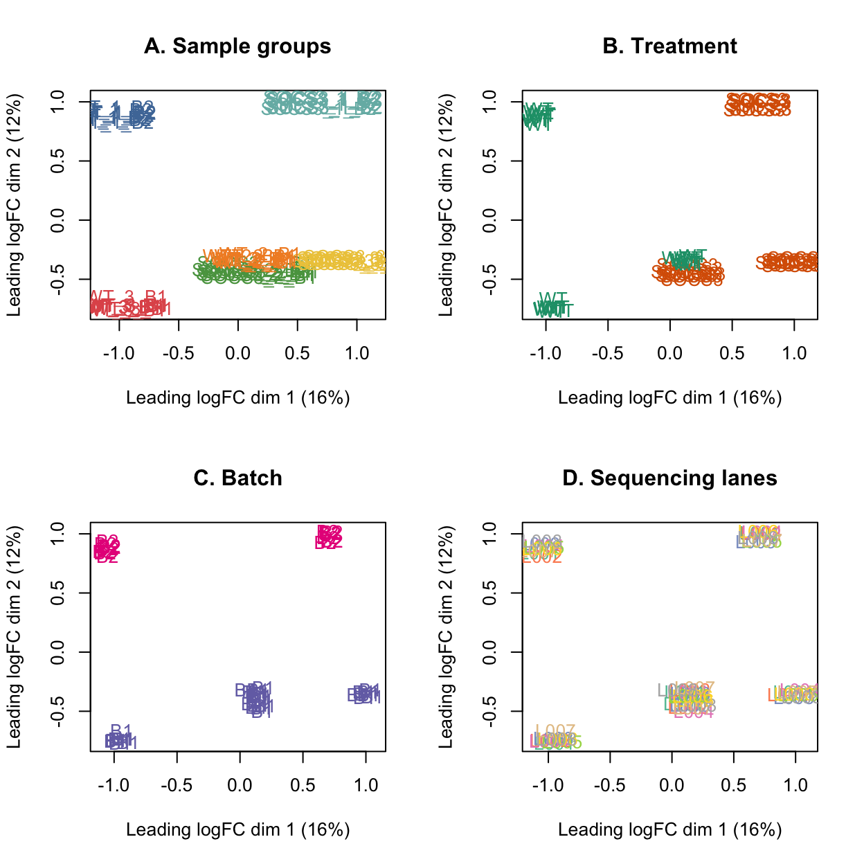
MDS plot with the library size overlayed on the samples shows that the samples from batch 2 have a much lower library size than the samples from batch 1. It also shows that the sample which does not follow the trend observed for the treatment has a low library size, so this may be due to low quality samples.
Show code
par(mfrow = c(2,2))
plotMDS(lcpm, labels=group, col=group_colours[group])
title(main="A. Sample groups")

plotMDS(lcpm, labels=treatment, col=treatment_colours[treatment])
title(main="B. Treatment")

plotMDS(lcpm, labels=batch, col=batch_colours[batch])
title(main="C. Batch")

# MDS plot with library size
libsizes <- dge$samples$lib.size

# Create a viridis color function
color_func <- scales::col_numeric(viridis::viridis(100), domain = range(libsizes))

# Assign colors according to library sizes
point_colors <- color_func(libsizes)

plotMDS(lcpm, labels=NULL, pch = 16, cex = 4, col=point_colors)
title(main="D. Library Size") 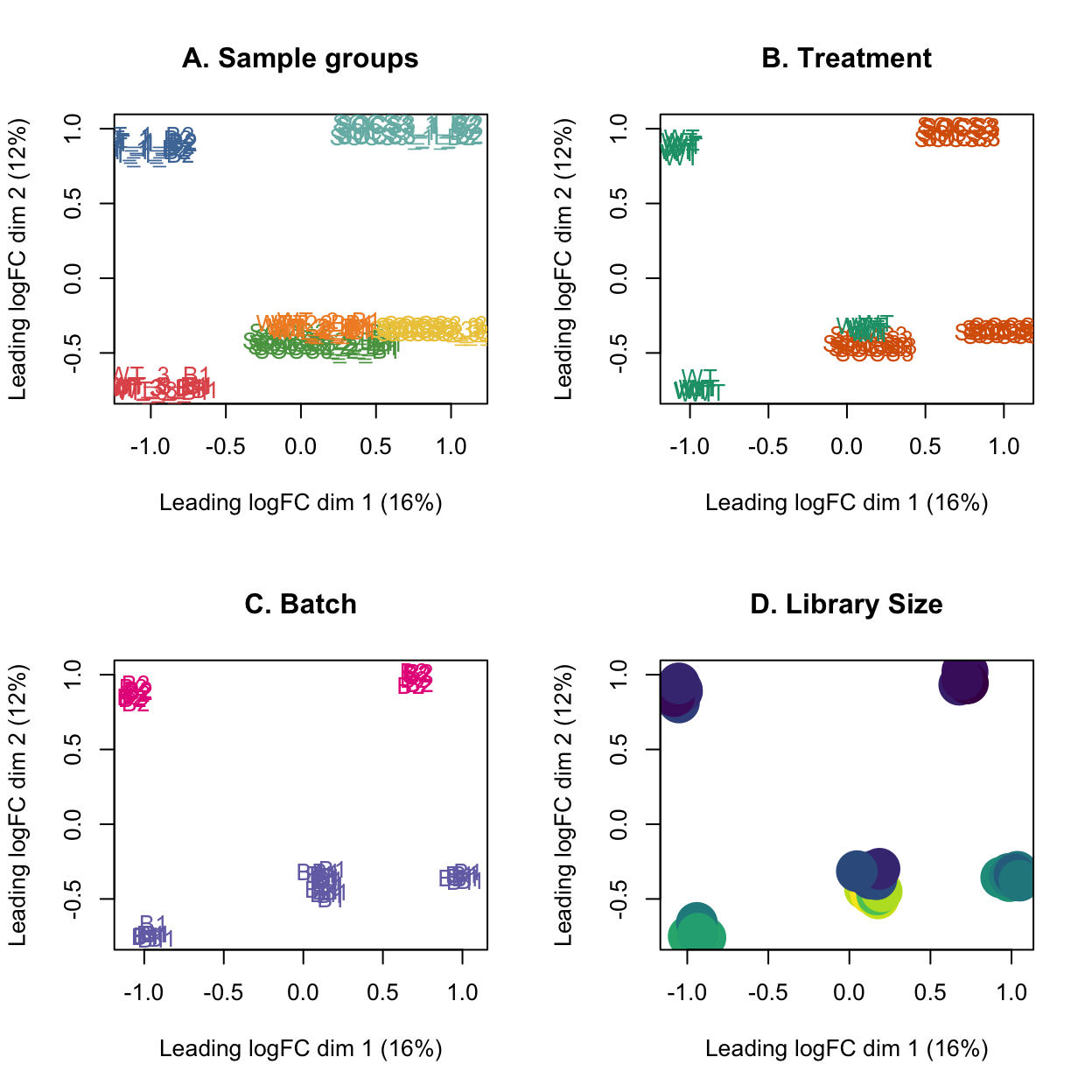
This plot shows that the third and fourth principal components show some separation by treatment, and still some trend from library size. The batch effect is primarily in the first two principal components.
Show code
# MDS plots of the third and fourth dimension
par(mfrow=c(2,2))
plotMDS(lcpm, labels=group, col=group_colours[group], dim=c(3,4))
title(main="A. Sample groups")

plotMDS(lcpm, labels=treatment, col=treatment_colours[treatment], dim=c(3,4))
title(main="B. Treatment")

plotMDS(lcpm, labels=batch, col=batch_colours[batch], dim=c(3,4))
title(main="C. Batch")

# MDS plot with library size
libsizes <- dge$samples$lib.size

# Create a viridis color function
color_func <- scales::col_numeric(viridis::viridis(100), domain = range(libsizes))

# Assign colors according to library sizes
point_colors <- color_func(libsizes)

plotMDS(lcpm, labels=NULL, pch = 16, cex = 4, col=point_colors, dim=c(3,4))
title(main="D. Library Size") 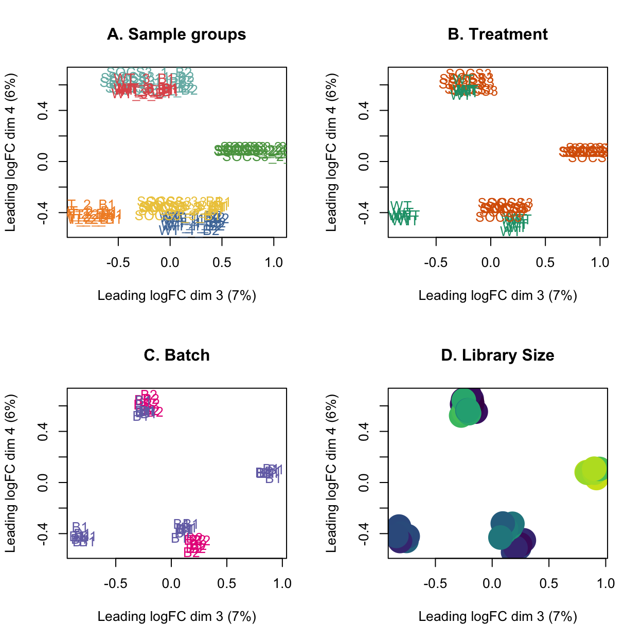
Comparing batches for genes of interest
Show code
genes_of_interest <- c("Socs3", "Socs1", "Bcl3")
selected_genes <- grep(glue::glue_collapse(genes_of_interest, "|"), dge$genes$SYMBOL)

cpm_agg <- edgeR::cpm(dge)
lcpm_agg <- edgeR::cpm(dge, log=TRUE)
df <- data.frame(
    y = t(lcpm_agg[selected_genes, ]),
    treatment = dge$samples$treatment,
    batch = dge$samples$batch)

# NOTE: The order of the columns corresponds to the order of these genes in the
#   rownames, NOT the order that was listed in genes_of_interest.
colnames(df)[1:3] <- gsub("y.", "", colnames(df)[1:3])

df$labels <- factor(paste0(df$batch, ".", df$treatment),
    levels=c("B1.WT", "B1.SOCS3", "B2.WT", "B2.SOCS3"))

plot_list <- list()
for (i in 1:3) {
    plot_list[[i]] <-
        ggplot(data = df, mapping = aes(x = labels, y = .data[[genes_of_interest[i]]], group = labels, colour = treatment)) +
            geom_point(size = 4) +
            theme_minimal() +
            theme(axis.text.x = element_text(angle = 45, hjust = 1)) +
            ylab("Expression (log CPM)") +
            scale_colour_manual(values = treatment_colours) +
            ggtitle(label = paste0(genes_of_interest[i])
    )
}
patchwork::wrap_plots(plot_list, ncol = 3, guides = "collect") 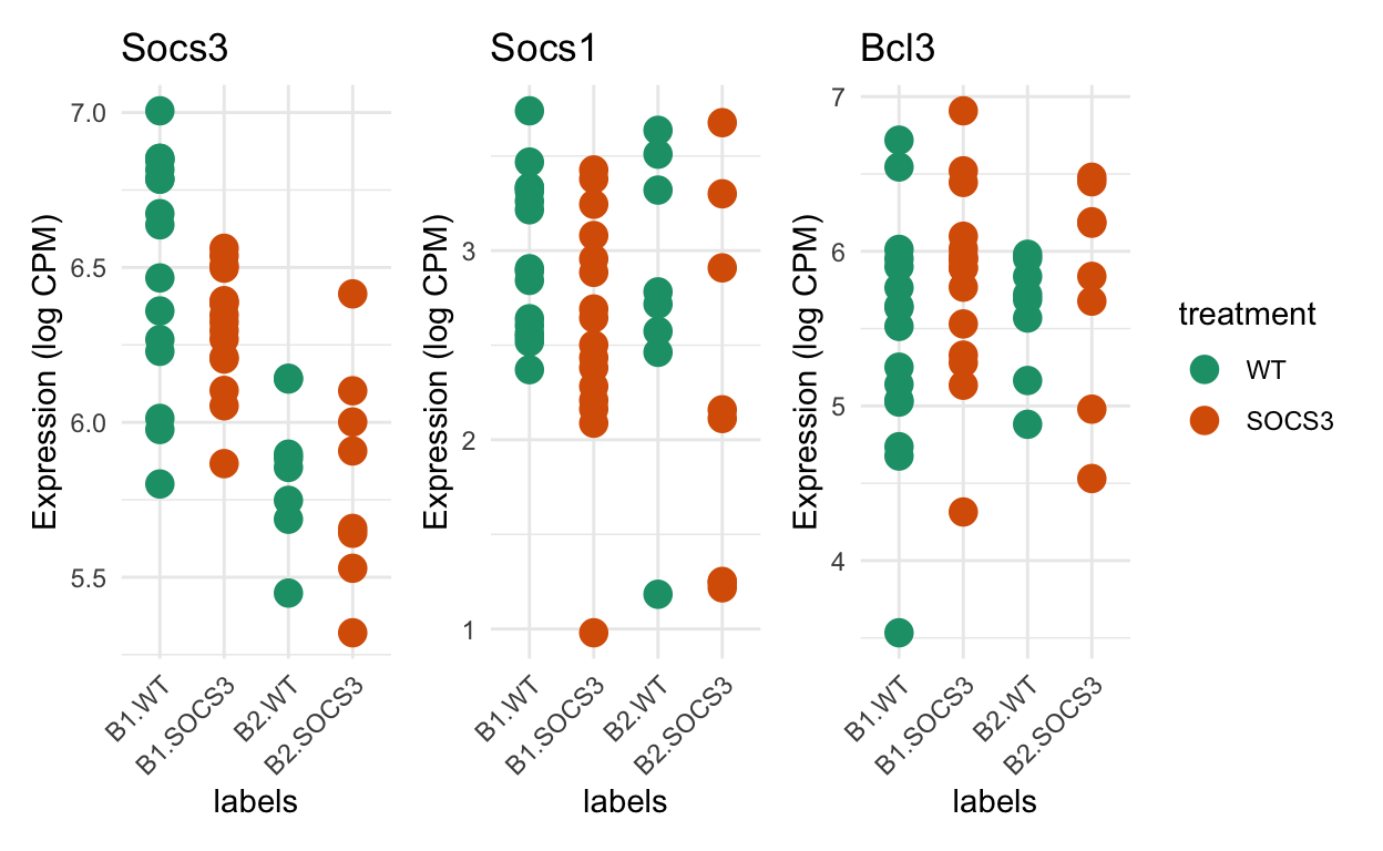
Differential Expression Analyses
At the lane-based level, performing DE analyses will lead to pseudo-replicates.
The 8 lanes for a particular sample are not independent.
If we instead had different mice in each lane as in the RNA-seq is as easy as 123 paper, we could include lane as a covariate.
Conclusion
Based on the MDS plots, the technical replicates from the same sample are quite similar. The best way to perform this analysis is to concatenate the FastQ files from the same samples in the very beginning of the analysis.