Introduction

This report includes an analysis of the Socs3 knockout bulk RNA-sequencing data. The data includes 6 samples, 3 from the control group (wild-type) and 3 from the Socs3 knockout group. The samples are from bone tissue of mice (and some samples contain multiple mice). We are interested in seeing if there are differences in gene expression between these groups, as this will help to understand the role of Socs3.

The gene filtering, normalisation, MDS plot and differential expression testing is based on the guide “RNA-seq analysis is easy as 1-2-3 with limma, Glimma and edgeR” (Law et al. 2018), see https://pmc.ncbi.nlm.nih.gov/articles/PMC4937821/.

Show code

# Load required libraries for the document 
library(here)
library(tximport)
library(biomaRt)
library(edgeR)
library(patchwork)
library(limma) 
library(RColorBrewer) 
library(ggplot2) 
library(gridExtra) 
library(dplyr)
library(pheatmap)

Setting up the data

There are a number of pre-processing steps required to obtain a count matrix of this data. First, the .fastq files from the same sample and read combination were merged together (see code/03_merge_lanes.sh. There are 6 samples so this results in 12 .fastq files (read 1 and read 2 for each sample).

Next, the paired-end reads were aligned to the reference mouse transcriptome using kallisto.

Reading in count data

Since kallisto uses transcript IDs instead of gene IDs, we will use the biomaRt package to map transcript IDs to gene IDs. When we import the data using tximport, the transcripts are aggregated at the gene level using this mapping.

Show code

samples_output <- list.files(here("data/kallisto"))

# Get this to work and look at the files
file_paths <- here("data/kallisto/", samples_output, "abundance.h5")
names(file_paths) <- gsub("_output", "", samples_output)

# Use biomaRt to map transcripts to gene_ids
mart <- useMart("ensembl", dataset = "mmusculus_gene_ensembl", verbose = TRUE)

BioMartServer running BioMart version: 0.7
Mart virtual schema: default
Mart host: https://www.ensembl.org:443/biomart/martservice

Show code

transcript_map <- getBM(
  attributes = c("ensembl_transcript_id",
                 "ensembl_gene_id",
                 "external_gene_name",
                 "chromosome_name"),
  mart = mart
)

txi.kallisto <- tximport(
    file_paths, 
    type = "kallisto", 
    txOut = FALSE,
    tx2gene = transcript_map[, c("ensembl_transcript_id", "ensembl_gene_id")],
    ignoreTxVersion = TRUE
    )

Next, we create a DGEList object from the count data and the sample sheet. The count data contains a column for each sample of the experiment (6 in total). The sample sheet (located in data/sample_sheet.csv) includes information about the mouse genotype, the batches, and other experimental information.

The DGEList object includes counts for the numeric data, and the samples and genes data frames, which contains information about the samples and features, respectively.

Show code

# Read in count data
counts <- txi.kallisto$counts

# Subset the transcript_map to match our data
dim(transcript_map)
gene_info <- transcript_map[match(row.names(counts), transcript_map$ensembl_gene_id), ]
dim(gene_info)

gene_info$CHR <- gene_info$chromosome_name
gene_info$SYMBOL <- gene_info$external_gene_name
gene_info$ENSEMBL <- gene_info$ensembl_gene_id

There are 36091 genes currently in the object.

Show code

# Read in sample sheet
samples <- read.csv(here("data/sample_sheet.csv"), row.names = 1)

colnames(counts) <- gsub("_22YMFCLT3", "", colnames(counts))

# The sample sheet is already in the correct order
stopifnot(identical(samples$Sample_name, colnames(counts)))

colnames(counts) <- samples$group

Kallisto mapping information

The table below shows the percentage of reads which are mapped. This mapping rate looks okay.

Show code

library(jsonlite)

# Path to each kallisto folder
sample_dirs <- dirname(file_paths)

# Extract mapping rate from run_info.json for each sample
mapping_rates <- sapply(sample_dirs, function(dir) {
  info <- fromJSON(file.path(dir, "run_info.json"))
  info$p_pseudoaligned
}) / 100

df <- data.frame(
    File = gsub("_22YMFCLT3_output", "", basename(sample_dirs)),
    Mapping_rate = mapping_rates)
df$Group <- samples$group[match(df$File, samples$Sample_name)]

rownames(df) <- NULL
df[, c("Group", "Mapping_rate")]|> 
    janitor::adorn_pct_formatting() |>
    knitr::kable()

Group	Mapping_rate
WT_1_B2	53.8%
SOCS3_1_B2	49.6%
SOCS3_2_B1	73.0%
SOCS3_3_B1	63.7%
WT_2_B1	64.8%
WT_3_B1	73.0%

Next we create a DGEList from the count data and the sample sheet. The count data contains a column for each sample of the experiment (6 in total). The sample sheet includes information about the mouse genotype and the batches.

The DGEList object includes counts for the numeric data, and the samples and genes data frames, which contains information about the samples and features, respectively.

Show code

# Create the DGEList. 
dge <- DGEList(
    counts, 
    samples = samples, 
    group = samples$group, 
    genes = gene_info)
dim(dge)

[1] 36091     6

Organising sample information

Show code

group <- dge$samples$group
batch <- gsub(".+_", "", dge$samples$group)
treatment <- gsub("_.+", "", dge$samples$group)

# Make sample info factors
group <- factor(group, levels=c("WT_1_B2", "WT_2_B1", "WT_3_B1", 
    "SOCS3_1_B2", "SOCS3_2_B1", "SOCS3_3_B1"))
batch <- factor(batch)
treatment <- factor(treatment, levels=c("WT", "SOCS3"))

# Add sample info into samples slot. 
dge$samples$batch <- batch
dge$samples$treatment <- treatment

There are 6 samples, 3 for each treatment.

Show code

table(group, treatment)

            treatment
group        WT SOCS3
  WT_1_B2     1     0
  WT_2_B1     1     0
  WT_3_B1     1     0
  SOCS3_1_B2  0     1
  SOCS3_2_B1  0     1
  SOCS3_3_B1  0     1

Show code

# Remove group, treatment and batch. These should only be accessed from dge!!!
rm(group, batch, treatment)

Organising gene annotations

After mapping the sequencing reads to the transcriptome, we have Ensembl-style transcript identifiers. These are used by mapping tools as they are unambiguous and highly stable. We have used the biomaRt package to match these transcript IDs to gene IDs. From the gene IDs, we also obtain gene symbols and chromosome information, for easier interpretation of the results.

Show code

# There are hundreds of duplicate symbols.
table(duplicated(gene_info$SYMBOL))
# No duplicate ENSEMBL id's now. 
table(duplicated(gene_info$ENSEMBL))

There are some Ensembl IDs which map to the same gene symbols. For these features we will refer to the genes using both the Ensembl ID and the symbol, for example “Pakap_ENSMUSG00000038729.25”. This ensures that rownames are unique, giving us a robust way of subsetting the object and referring to genes in the analysis.

Show code

library(scuttle)

rownames(dge) <- uniquifyFeatureNames(dge$genes$ENSEMBL, dge$genes$SYMBOL)
# Duplicate features with symbols have their ID concatenated.  
# rownames(dge)[duplicated(dge$genes$SYMBOL) & !is.na(dge$genes$SYMBOL)]
# Now there are unique rownames. 
table(duplicated(rownames(dge)))

We save the DGEList object to file, located at data/kallisto.dge.rds.

Show code

saveRDS(dge, here("data/kallisto.dge.rds"))
dge <- readRDS(here("data/kallisto.dge.rds"))

We remove features which aren’t expressed in any samples of our data.

In doing this we also check that this have not removed any of our genes of interest, which include Socs1, Socs3 and Bcl3. Reassuringly, these features are not removed during this step and thus have some expression in the data.

Show code

genes_of_interest <- c("Socs1", "Socs3", "Bcl3")
# genes of interest are in our rownames originally
genes_of_interest %in% dge$genes$SYMBOL

[1] TRUE TRUE TRUE

Show code

# Remove genes expressed in no samples. 
dge_zeroes <- dge[(rowSums(dge$counts) == 0), ]

# See if any of our genes of interest are not being expressed
genes_of_interest %in% dge_zeroes$genes$SYMBOL

[1] FALSE FALSE FALSE

Show code

# Remove features which aren't expressed in any samples. 
dge <- dge[(rowSums(dge$counts) > 0), ]

There are 8905 genes which aren’t expressed in any of the samples. These will be removed by any filtering metric that we choose to use. There are 27186 genes remaining for analysis.

Pre-processing

Show code

# NOTE: Annoyingly, my cpm function is being masked by SingleCellExperiment. 
# Having to specify the edgeR package to get this line to work. 
# Transform from raw scale
cpm <- edgeR::cpm(dge)
lcpm <- edgeR::cpm(dge, log=TRUE)

Show code

keep.exprs <- filterByExpr(dge, group=dge$samples$group)
dge <- dge[keep.exprs,, keep.lib.sizes=FALSE]
dim(dge)
# This function keeps genes with about 10 read counts or more in a minimum
# number of samples.
sum(keep.exprs == FALSE)

Filtering using FilterByExpr from the edgeR package removes genes with very low expression. There are 5414 genes which are removed due to having low expression. There are 21772 genes remaining for analysis.

These low quality genes result in a spike near 0 in the left-hand side of the plot below. In the filtered data, the lowly expressed genes are mostly removed. The samples have a similar distribution of genes in this plot.

Show code

# Figure 1: Density of the raw post filtered data

# M is the mean, L is the median
L <- mean(dge$samples$lib.size) * 1e-6
M <- median(dge$samples$lib.size) * 1e-6

lcpm.cutoff <- log2(10/M + 2/L)
library(RColorBrewer)
nsamples <- length(unique(dge$samples$group))
col <- brewer.pal(nsamples, "Paired")
par(mfrow=c(1,2))
plot(density(lcpm[,1]), col=col[1], lwd=2, ylim=c(0,0.26), las=2, main="", xlab="")
title(main="A. Raw data", xlab="Log-cpm")
abline(v=lcpm.cutoff, lty=3)
for (i in 2:nsamples){
  den <- density(lcpm[,i])
  lines(den$x, den$y, col=col[i], lwd=2)
}
legend("topright", as.character(unique(dge$samples$group)), text.col=col, bty="n")
lcpm <- edgeR::cpm(dge, log=TRUE)
plot(density(lcpm[,1]), col=col[1], lwd=2, ylim=c(0,0.26), las=2, main="", xlab="")
title(main="B. Filtered data", xlab="Log-cpm")
abline(v=lcpm.cutoff, lty=3)
for (i in 2:nsamples){
  den <- density(lcpm[,i])
  lines(den$x, den$y, col=col[i], lwd=2)
}
legend("topright", as.character(unique(dge$samples$group)), text.col=col, bty="n")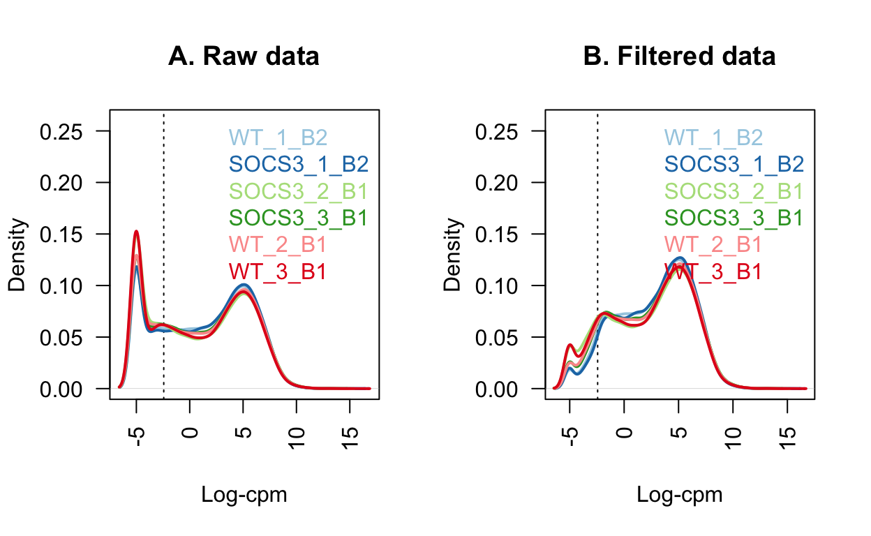

Quality control

Show code

# Set colours for this data set
group_colours <- setNames(
    ggthemes::tableau_color_pal("Tableau 10")(6), 
    levels(dge$samples$group))

batch_colours <- setNames(
    brewer.pal(8, "Dark2")[3:4], 
    levels(dge$samples$batch))

treatment_colours <- setNames(
    brewer.pal(8, "Dark2")[1:2], 
    levels(dge$samples$treatment))

Library size

The bar charts below show the library sizes for each sample, coloured by sample, batch and treatment. The samples from batch 2 have smaller library sizes on average than the batch 1 samples. The sample WT_2_B1 from batch 1 also has a small library size.

Show code

# this factor ordering for group is helpful for QC, as it puts everything from 
# the same batch next to each other. 
dge$samples$group <- factor(dge$samples$group,
    levels = c("WT_2_B1", "WT_3_B1", "SOCS3_2_B1", "SOCS3_3_B1", "WT_1_B2", "SOCS3_1_B2"))

p1 <- ggplot(data = dge$samples, mapping = aes(y = group, x = lib.size, fill = group)) + 
    geom_col() +
    scale_fill_manual(values = group_colours) +
    scale_y_discrete(limits = rev(levels(dge$samples$group))) +
    theme_minimal()
p2 <- ggplot(data = dge$samples, mapping = aes(y = group, x = lib.size, fill = batch)) + 
    geom_col() +
    scale_fill_manual(values = batch_colours) +
    scale_y_discrete(limits = rev(levels(dge$samples$group))) +
    theme_minimal()
p3 <- ggplot(data = dge$samples, mapping = aes(y = group, x = lib.size, fill = treatment)) + 
    geom_col() +
    scale_fill_manual(values = treatment_colours) + 
    scale_y_discrete(limits = rev(levels(dge$samples$group))) +
    theme_minimal()
(p1 / p2 / p3) + plot_layout(guides = "collect")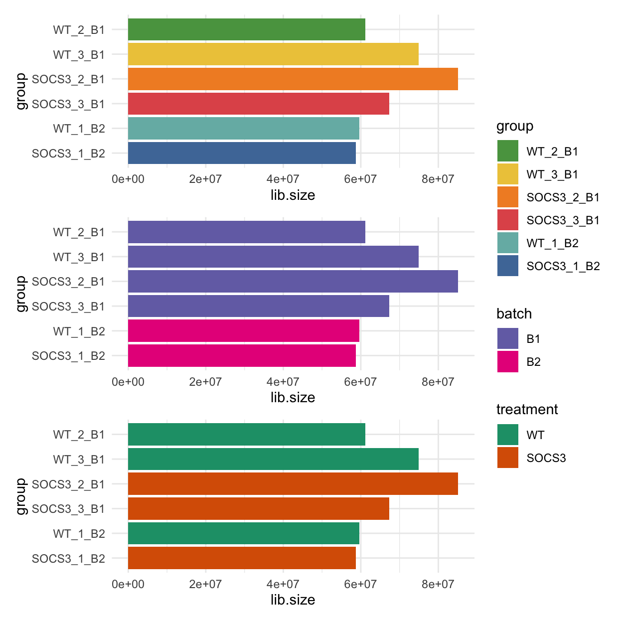

We can also look at some other experimental variables that could explain the different library sizes. The bar charts below are coloured by the number of mice used, and the concentration of RNA. Since the batch 2 samples only had one mice each, this could explain the lower library size for these samples. The concentration also has a moderate correlation with the library size.

Show code

stopifnot(identical(colnames(dge), c("WT_1_B2", "SOCS3_1_B2", "SOCS3_2_B1", "SOCS3_3_B1", "WT_2_B1", "WT_3_B1")))
dge$samples$nMice <- factor(c(1, 1, 3, 2, 3, 2))

Show code

p1 <- ggplot(data = dge$samples, mapping = aes(y = group, x = lib.size, fill = group)) + 
    geom_col() +
    scale_fill_manual(values = group_colours) +
    scale_y_discrete(limits = rev(levels(dge$samples$group))) +
    theme_minimal()
p2 <- ggplot(data = dge$samples, mapping = aes(y = group, x = lib.size, fill = nMice)) + 
  geom_col() +
  scale_y_discrete(limits = rev(levels(dge$samples$group))) +
  scale_fill_manual(
    values = c("1" = "#6a51a3", "2" = "#c09be6", "3" = "#f2e5ff"),
    name = "Number of Mice"
  ) +
  theme_minimal()
p3 <- ggplot(data = dge$samples, mapping = aes(y = group, x = lib.size, fill = Concentration)) + 
    geom_col() +
    scale_y_discrete(limits = rev(levels(dge$samples$group))) +
    theme_minimal()
(p1 / p2 / p3) + plot_layout(guides = "collect")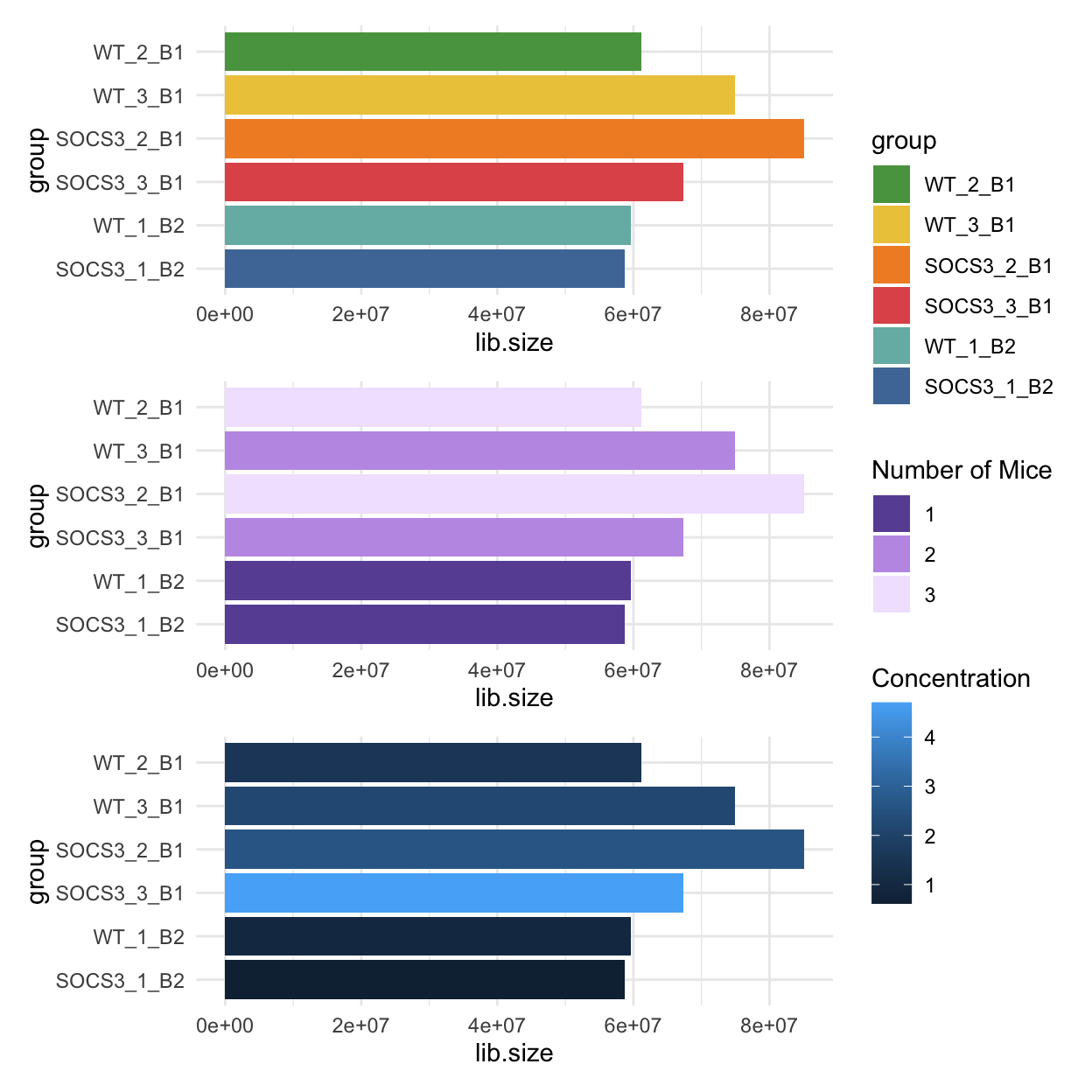

Show code

library(ggpubr)

ggplot(dge$samples, aes(x = Concentration, y = lib.size)) +
  geom_point() +
  stat_cor(method = "pearson") +
  theme_light()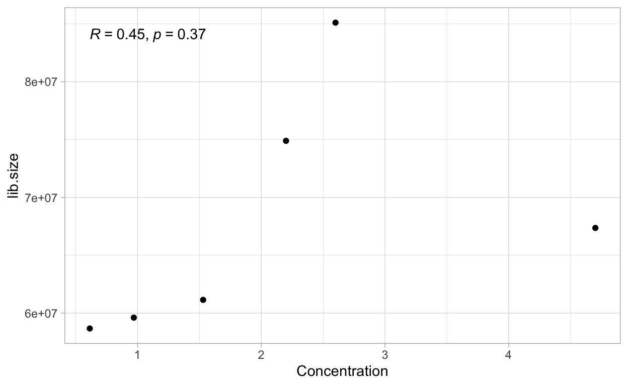

Number of expressed features

Expressed features are defined as those with at least one count in a sample. There is a similar number of expressed features in each sample. Each sample has around 20,000 genes with at least one count.

Show code

dge$samples$nFeatures <- apply(dge$counts, MARGIN = 2, FUN = function(x) {sum(x > 0)})

dge$samples |>
    dplyr::select(group, nFeatures) |>
    knitr::kable()

	group	nFeatures
WT_1_B2	WT_1_B2	21414
SOCS3_1_B2	SOCS3_1_B2	21375
SOCS3_2_B1	SOCS3_2_B1	20939
SOCS3_3_B1	SOCS3_3_B1	21250
WT_2_B1	WT_2_B1	21272
WT_3_B1	WT_3_B1	20876

Proportion of mitochondrial genes

Show code

table(dge$genes$CHR)


         1         10         11         12         13         14 
      1302       1027       1621        886        876        873 
        15         16         17         18         19          2 
       804        678       1088        539        694       1715 
         3          4          5          6          7          8 
      1012       1281       1263       1260       1772       1022 
         9 GL456210.1 GL456211.1 GL456212.1 GL456221.1 JH584304.1 
      1202          3          3          2          5          1 
        MT          X          Y 
        13        793         37

Show code

mito_set <- rownames(dge$genes)[dge$genes$CHR == "MT"]

We can identify mitochondrial genes as genes with the chromosome number “MT”. There are 13 mitochondrial genes.

The chunk below works out the proportion of counts in each sample which are mitochondrial. High proportions of mitochondrial RNA can indicate that the cells in the sample are under stress. In this case, the proportion is very low (0.5-1.5%), which is good. There is however noticeably higher percentages in the batch2 data. There is no trend between treatment and mitochondrial proportion, which is good.

Show code

# Apply to each sample
dge$samples$mito_pct <- apply(dge$counts, MARGIN = 2, FUN = function(x) {sum(x[mito_set]) / sum(x)})

dge$samples |>
    dplyr::select(group, mito_pct) |>
    janitor::adorn_pct_formatting() |>
    knitr::kable()

	group	mito_pct
WT_1_B2	WT_1_B2	1.1%
SOCS3_1_B2	SOCS3_1_B2	1.2%
SOCS3_2_B1	SOCS3_2_B1	0.7%
SOCS3_3_B1	SOCS3_3_B1	0.6%
WT_2_B1	WT_2_B1	0.6%
WT_3_B1	WT_3_B1	0.5%

Show code

library(scales)

# No trends here
p1 <- ggplot(data = dge$samples, mapping = aes(y = group, x = mito_pct, fill = group)) + 
    geom_col() +
    scale_fill_manual(values = group_colours) +
    scale_x_continuous(labels = label_percent()) +
    scale_y_discrete(limits = rev(levels(dge$samples$group))) +
    theme_minimal()
p2 <- ggplot(data = dge$samples, mapping = aes(y = group, x = mito_pct, fill = batch)) + 
    geom_col() +
    scale_fill_manual(values = batch_colours) +
    scale_x_continuous(labels = label_percent()) +
    scale_y_discrete(limits = rev(levels(dge$samples$group))) +
    theme_minimal()
p3 <- ggplot(data = dge$samples, mapping = aes(y = group, x = mito_pct, fill = treatment)) + 
    geom_col() +
    scale_fill_manual(values = treatment_colours) + 
    scale_x_continuous(labels = label_percent()) +
    scale_y_discrete(limits = rev(levels(dge$samples$group))) +
    theme_minimal()
(p1 / p2 / p3) + plot_layout(guides = "collect")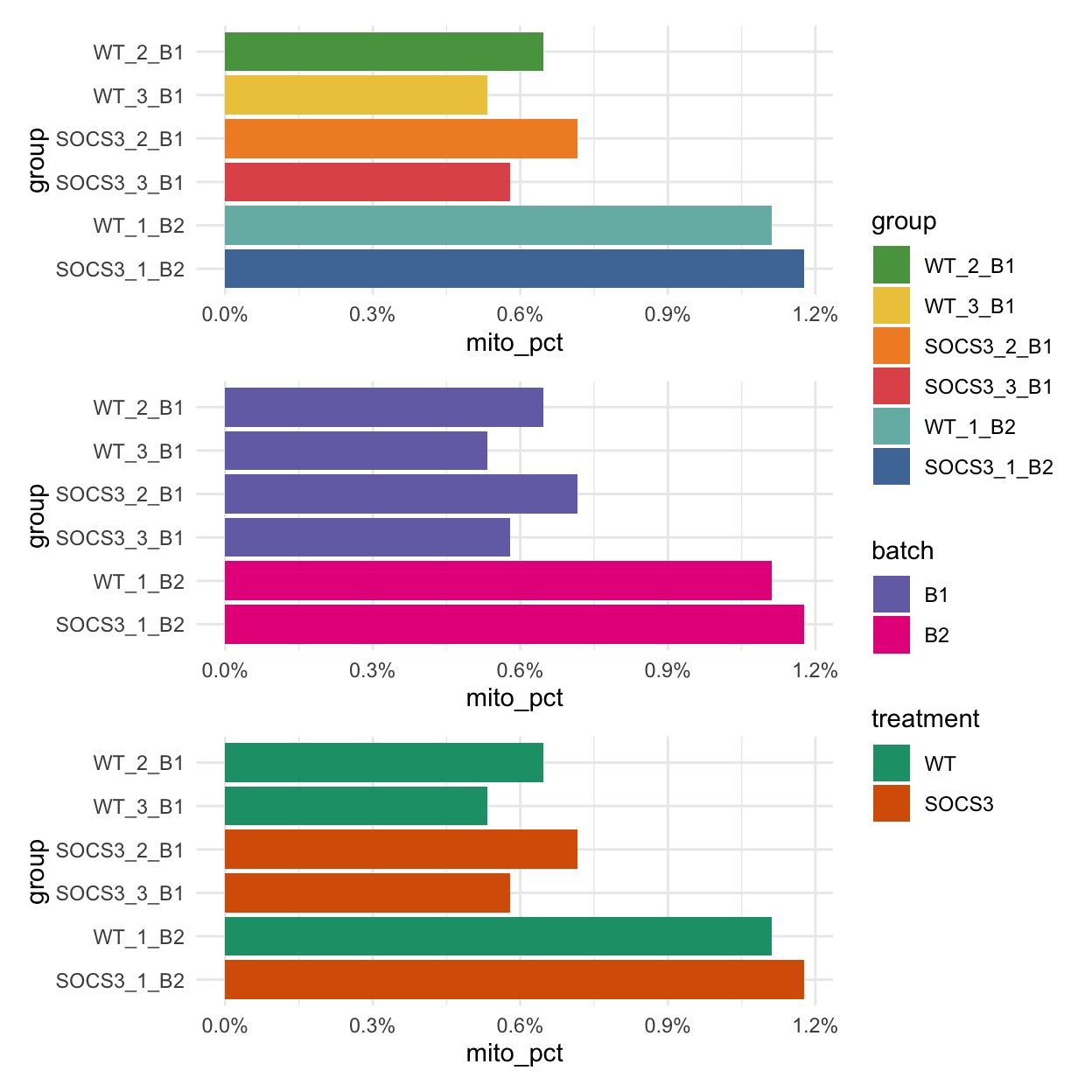

Normalisation

The impact of normalisation is subtle. Most notably, the third quartiles have been brought into alignment.

Show code

dge_raw <- dge
dge <- calcNormFactors(dge, method = "TMM")

The library sizes for the samples are listed in the table below. This is the sum of counts across every gene for each sample. The counts in the Hisat2 analysis were roughly 10 million per sample, and the kallisto analysis has about 60 million counts per sample. Possibly this is due to the way each method handles PCR duplicates as well as some reads not mapping in the hisat2 version.

Show code

# Library sizes
dge_raw$sample |> 
    dplyr::select(lib.size) |>
    knitr::kable(col.names = c("Sample", "Library size"))

Sample	Library size
WT_1_B2	59608523
SOCS3_1_B2	58669677
SOCS3_2_B1	85103114
SOCS3_3_B1	67361444
WT_2_B1	61145081
WT_3_B1	74887905

Show code

# log-cpm in appropriate order for plot
# NOTE: NEVER USE WITH dge$samples!!! For plotting only!!
lcpm_raw_plot <- edgeR::cpm(dge_raw, log=TRUE)[, levels(dge_raw$samples$group)]
lcpm_plot <- edgeR::cpm(dge, log = TRUE)[, levels(dge$samples$group)]

# y-limit for plot 
ylims <- range(c(lcpm_raw_plot, lcpm_plot))
par(mfrow=c(1,2))

boxplot(lcpm_raw_plot, las=2, col=col, main="", )
title(main="A. Example: Unnormalised data", ylab="Log-cpm")

boxplot(lcpm_plot, las=2, col=col, main="")
title(main="B. Example: Normalised data", ylab="Log-cpm")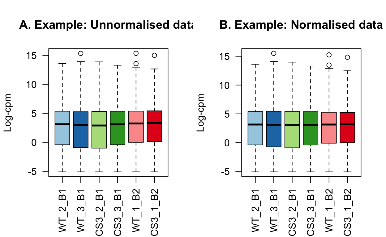

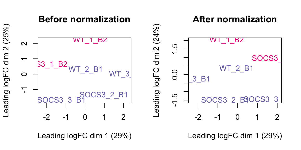
The plots below show the MDS plot before and after normalisation. This has a more obvious difference than the boxplot above.

Show code

par(mfrow = c(1,2))
plotMDS(dge_raw, main="Before normalization", col=batch_colours[dge_raw$samples$batch])
plotMDS(dge, main="After normalization", col=batch_colours[dge$samples$batch])

After normalising the data, we need to evaluate the log counts again.

Show code

cpm <- edgeR::cpm(dge)
lcpm <- edgeR::cpm(dge, log=TRUE)

Visualising the data

MDS plot with the library size overlayed on the samples shows that the samples from batch 2 have lower library sizes than the samples from batch 1. The sample WT_2_B1 clusters in the centre of the data which may indicate that it has different expression profiles to both the WT and SOCS3 samples. It also has a low library size.

Show code

par(mfrow = c(2,2))
plotMDS(lcpm, labels=dge$samples$group, col=group_colours[dge$samples$group])
title(main="A. Sample groups")

plotMDS(lcpm, labels=dge$samples$treatment, col=treatment_colours[dge$samples$treatment])
title(main="B. Treatment")

plotMDS(lcpm, labels=dge$samples$batch, col=batch_colours[dge$samples$batch])
title(main="C. Batch")

# MDS plot with library size
libsizes <- dge$samples$lib.size

# Create a viridis color function
color_func <- scales::col_numeric(viridis::viridis(100), domain = range(libsizes))

# Assign colors according to library sizes
point_colors <- color_func(libsizes)

plotMDS(lcpm, labels=NULL, pch = 16, cex = 4, col=point_colors)
title(main="D. Library Size")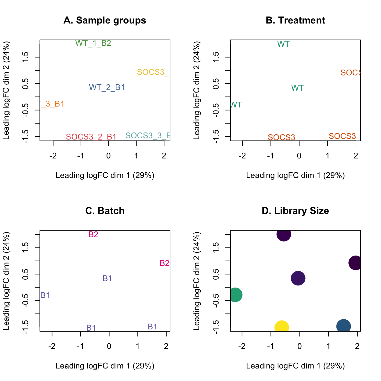

Comparing batches for genes of interest

The plots below show the expression of three of our genes of interest. Based on a priori knowledge, the SOCS3 knockout samples should express Socs1 and Socs3 less than the WT. Bcl3 should be higher in the SOCS3 group. The difference in these 6 samples is small and will not come out as significant in DE testing.

Show code

genes_of_interest <- c("Socs3", "Socs1", "Bcl3")
selected_genes <- grep(glue::glue_collapse(genes_of_interest, "|"), dge$genes$SYMBOL)

cpm <- edgeR::cpm(dge)
lcpm <- edgeR::cpm(dge, log=TRUE)
df <- data.frame(
    y = t(lcpm[selected_genes, ]), 
    treatment = dge$samples$treatment, 
    batch = dge$samples$batch)

# NOTE: The order of the columns corresponds to the order of these genes in the 
#   rownames, NOT the order that was listed in genes_of_interest.
colnames(df)[1:3] <- gsub("y.", "", colnames(df)[1:3])

df$labels <- factor(paste0(df$batch, ".", df$treatment),
    levels=c("B1.WT", "B1.SOCS3", "B2.WT", "B2.SOCS3"))

plot_list <- list()
for (i in 1:3) {
    plot_list[[i]] <-
        ggplot(data = df, mapping = aes(x = labels, y = .data[[genes_of_interest[i]]], group = labels, colour = treatment)) + 
            geom_point(size = 4) + 
            theme_minimal() + 
            theme(axis.text.x = element_text(angle = 45, hjust = 1)) + 
            ylab("Expression (log CPM)") + 
            scale_colour_manual(values = treatment_colours) +
            ggtitle(label = paste0(genes_of_interest[i])
    )
}
patchwork::wrap_plots(plot_list, ncol = 3, guides = "collect")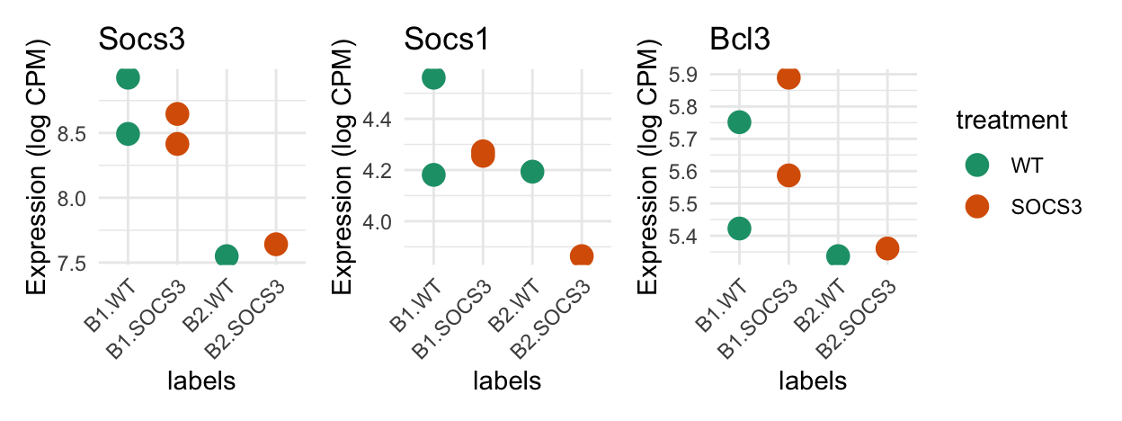

Show code

# Table format
lcpm[selected_genes, ] |>
    as.data.frame() |>
    tibble::rownames_to_column("ENSEMBL") |>
    dplyr::mutate(SYMBOL = dge$genes$SYMBOL[selected_genes], .after = "ENSEMBL")

  ENSEMBL SYMBOL  WT_1_B2 SOCS3_1_B2 SOCS3_2_B1 SOCS3_3_B1  WT_2_B1
1   Socs1  Socs1 4.193607   3.863719   4.273091   4.255331 4.560619
2   Socs3  Socs3 7.550153   7.641535   8.646510   8.415269 8.926129
3    Bcl3   Bcl3 5.337065   5.360624   5.889254   5.586850 5.751546
   WT_3_B1
1 4.181088
2 8.492555
3 5.422480

Differential Expression Analyses

We will be including 21772 genes in our differential expression analyses. Due to the high number of tests being performed, it is very important to use some form of multiple testing correction such as the False Discovery Rate (FDR). When performing tens of thousands of tests, there will be many significant genes (p-value < 0.05) even if there are no real differences between the treatments. Multiple testing correction makes the threshold for p-values stricter to account for this.

Treatment with limma::voom method

Since there is a strong batch effect, we will include batch as a covariate in the differential expression analysis. The analysis below uses the limma::voom() method for differential expression testing.

Show code

design <- model.matrix(~0+treatment+batch, data = dge$samples)

colnames(design) <- gsub("treatment|batch", "", colnames(design))

contr.matrix <- makeContrasts(
   SOCS3vsWT = SOCS3 - WT,
   levels = colnames(design))
contr.matrix

       Contrasts
Levels  SOCS3vsWT
  WT           -1
  SOCS3         1
  B2            0

Show code

v <- voom(dge, design, plot=TRUE)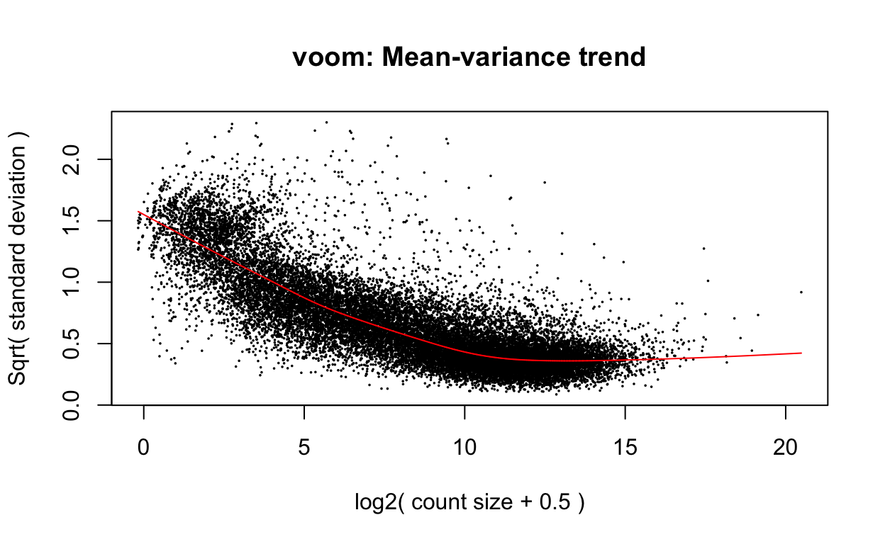

Show code

vfit <- lmFit(v, design)
vfit <- contrasts.fit(vfit, contrasts=contr.matrix)

efit <- eBayes(vfit)
plotSA(efit)

Show code

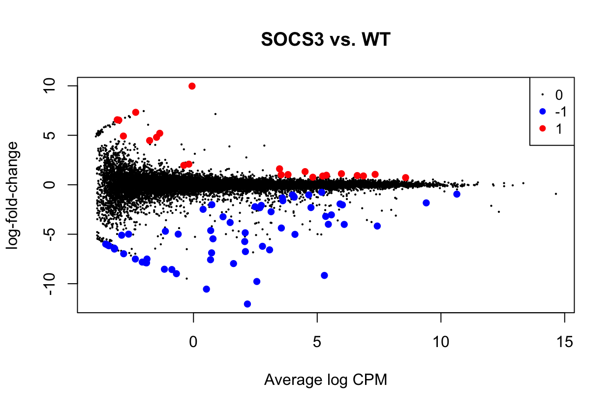
de_results <- decideTests(efit)

There is only one DE gene, and it is the immunoglobulin gene Igkv10-96. The top 20 genes (ranked by multiple-testing adjusted p-value) also includes some other Ig genes.

These genes are related to B-cells, and often indicate contamination from immune cells. Assess if it makes sense biologically to see less immunoglobulin expression in the Socs3 samples.

Show code

summary(de_results)

       SOCS3vsWT
Down           1
NotSig     21771
Up             0

Show code

# Sort the top table by adjusted P value
de_table <- topTable(efit, number=Inf, sort.by="P")
sorted_de <- de_table[order(de_table$adj.P.Val), ]

head(sorted_de, n=20)

          ensembl_transcript_id    ensembl_gene_id external_gene_name
Ighv1-53     ENSMUST00000103523 ENSMUSG00000093894           Ighv1-53
Igkv10-96    ENSMUST00000103328 ENSMUSG00000094420          Igkv10-96
Col18a1      ENSMUST00000081654 ENSMUSG00000001435            Col18a1
Pla2g2d      ENSMUST00000030528 ENSMUSG00000041202            Pla2g2d
Ighv1-82     ENSMUST00000196991 ENSMUSG00000095127           Ighv1-82
Ighv3-6      ENSMUST00000195124 ENSMUSG00000076672            Ighv3-6
Igkv4-79     ENSMUST00000103342 ENSMUSG00000076541           Igkv4-79
Ighv5-4      ENSMUST00000103444 ENSMUSG00000095612            Ighv5-4
Kera         ENSMUST00000105286 ENSMUSG00000019932               Kera
Ptx4         ENSMUST00000054930 ENSMUSG00000044172               Ptx4
Serpina1d    ENSMUST00000078869 ENSMUSG00000071177          Serpina1d
Atp6v0d2     ENSMUST00000029900 ENSMUSG00000028238           Atp6v0d2
Scx          ENSMUST00000229271 ENSMUSG00000034161                Scx
Ighv2-2      ENSMUST00000103443 ENSMUSG00000096464            Ighv2-2
Adamts3      ENSMUST00000061427 ENSMUSG00000043635            Adamts3
Itk          ENSMUST00000020664 ENSMUSG00000020395                Itk
St18         ENSMUST00000140079 ENSMUSG00000033740               St18
Spon2        ENSMUST00000200884 ENSMUSG00000037379              Spon2
Serpina1a    ENSMUST00000072876 ENSMUSG00000066366          Serpina1a
Gm16867      ENSMUST00000183917 ENSMUSG00000093954            Gm16867
          chromosome_name CHR    SYMBOL            ENSEMBL      logFC
Ighv1-53               12  12  Ighv1-53 ENSMUSG00000093894 -4.0124141
Igkv10-96               6   6 Igkv10-96 ENSMUSG00000094420 -1.9378250
Col18a1                10  10   Col18a1 ENSMUSG00000001435  0.8990599
Pla2g2d                 4   4   Pla2g2d ENSMUSG00000041202  1.3628040
Ighv1-82               12  12  Ighv1-82 ENSMUSG00000095127 -2.4104646
Ighv3-6                12  12   Ighv3-6 ENSMUSG00000076672 -2.1316224
Igkv4-79                6   6  Igkv4-79 ENSMUSG00000076541 -8.5587333
Ighv5-4                12  12   Ighv5-4 ENSMUSG00000095612 -4.6985150
Kera                   10  10      Kera ENSMUSG00000019932  1.3713546
Ptx4                   17  17      Ptx4 ENSMUSG00000044172  1.7728906
Serpina1d              12  12 Serpina1d ENSMUSG00000071177 -8.9632740
Atp6v0d2                4   4  Atp6v0d2 ENSMUSG00000028238  0.8859395
Scx                    15  15       Scx ENSMUSG00000034161  0.9467223
Ighv2-2                12  12   Ighv2-2 ENSMUSG00000096464 -1.3168779
Adamts3                 5   5   Adamts3 ENSMUSG00000043635  0.8820399
Itk                    11  11       Itk ENSMUSG00000020395 -1.0334949
St18                    1   1      St18 ENSMUSG00000033740  1.0191991
Spon2                   5   5     Spon2 ENSMUSG00000037379  0.9688598
Serpina1a              12  12 Serpina1a ENSMUSG00000066366 -7.1386943
Gm16867                14  14   Gm16867 ENSMUSG00000093954  0.7835625
            AveExpr          t      P.Value  adj.P.Val           B
Ighv1-53   4.959076 -15.353987 9.758266e-07 0.02124570  3.97176427
Igkv10-96  5.608252 -11.850155 5.842989e-06 0.06360678  3.98972269
Col18a1    4.994588   9.083638 3.517068e-05 0.24273285  2.66188572
Pla2g2d    4.331964   8.659995 4.825114e-05 0.24273285  2.16152507
Ighv1-82   4.091629  -8.069133 7.670576e-05 0.24273285  1.73742654
Ighv3-6    5.559966  -7.996783 8.134194e-05 0.24273285  1.97373795
Igkv4-79  -2.865525  -7.924391 8.629903e-05 0.24273285 -4.03276623
Ighv5-4    2.046985  -7.884291 8.919083e-05 0.24273285 -0.56749900
Kera       4.484776   7.406839 1.334934e-04 0.32293529  1.54837431
Ptx4       2.414982   6.526239 2.973713e-04 0.64743689  0.39576299
Serpina1d -1.916314  -6.311802 3.658982e-04 0.66979123 -3.89348036
Atp6v0d2   6.733194   6.301115 3.697491e-04 0.66979123  0.69001177
Scx        2.755483   6.169555 4.210637e-04 0.66979123  0.07625135
Ighv2-2    3.877833  -6.080932 4.601085e-04 0.66979123  0.33740415
Adamts3    3.354136   6.007886 4.953433e-04 0.66979123  0.16487991
Itk        4.535894  -5.997187 5.007532e-04 0.66979123  0.34735917
St18       3.434900   5.954529 5.229860e-04 0.66979123  0.09974794
Spon2      3.673332   5.868768 5.710967e-04 0.69077324  0.12662941
Serpina1a -1.348386  -5.796686 6.153696e-04 0.70514881 -3.62160400
Gm16867    4.730063   5.633636 7.303374e-04 0.79032187  0.02506500

Show code

# Write to a file
dir.create(here("output/DEGs/kallisto_analysis"), recursive = TRUE)
write.table(sorted_de, file=here("output/DEGs/kallisto_analysis/kallisto_treatment_voom.tsv"),
            sep="\t", quote=FALSE, row.names=FALSE)

A table of the differential expression results are saved in output/DEGs/kallisto_analysis/kallisto_treatment_voom.tsv. The rows are sorted so the genes with the lowest adjusted p-value (FDR) are at the top.

The results of testing for our genes of interest are shown below.

Show code

# Results for the genes of interest are not significant
sorted_de[sorted_de$SYMBOL %in% genes_of_interest, ]

      ensembl_transcript_id    ensembl_gene_id external_gene_name
Socs1    ENSMUST00000229866 ENSMUSG00000038037              Socs1
Bcl3     ENSMUST00000135609 ENSMUSG00000053175               Bcl3
Socs3    ENSMUST00000054002 ENSMUSG00000053113              Socs3
      chromosome_name CHR SYMBOL            ENSEMBL       logFC
Socs1              16  16  Socs1 ENSMUSG00000038037 -0.16771833
Bcl3                7   7   Bcl3 ENSMUSG00000053175  0.11362070
Socs3              11  11  Socs3 ENSMUSG00000053113 -0.08669159
       AveExpr          t   P.Value adj.P.Val         B
Socs1 4.219505 -1.2222948 0.2603406 0.9998741 -5.393089
Bcl3  5.557284  0.8798906 0.4075070 0.9998741 -5.931607
Socs3 8.278582 -0.6141822 0.5581169 0.9998741 -6.163115

Plots of the most differentially expressed genes

Plots of the most differentially expressed genes to see if the test is doing what we want it to do. There are several Ig genes here, and a collagen gene.

Show code

top_genes <- head(rownames(sorted_de), n = 6)

selected_genes <- match(top_genes, rownames(dge))

df <- data.frame(
    y = t(lcpm[selected_genes, ]), 
    treatment = dge$samples$treatment, 
    batch = dge$samples$batch)

colnames(df)[1:length(top_genes)] <- rownames(dge)[selected_genes]

df$labels <- factor(paste0(df$batch, ".", df$treatment),
    levels=c("B1.WT", "B1.SOCS3", "B2.WT", "B2.SOCS3"))

plot_list <- list()
for (i in 1:length(top_genes)) {
    plot_list[[i]] <-
        ggplot(data = df, mapping = aes(x = labels, y = .data[[top_genes[i]]], group = labels, colour = treatment)) + 
            geom_point(size = 4) + 
            theme_minimal() + 
            theme(axis.text.x = element_text(angle = 45, hjust = 1)) + 
            ylab("Expression (log CPM)") + 
            scale_colour_manual(values = treatment_colours) +
            ggtitle(label = paste0(top_genes[i])
    )
}
patchwork::wrap_plots(plot_list, ncol = 3, guides = "collect")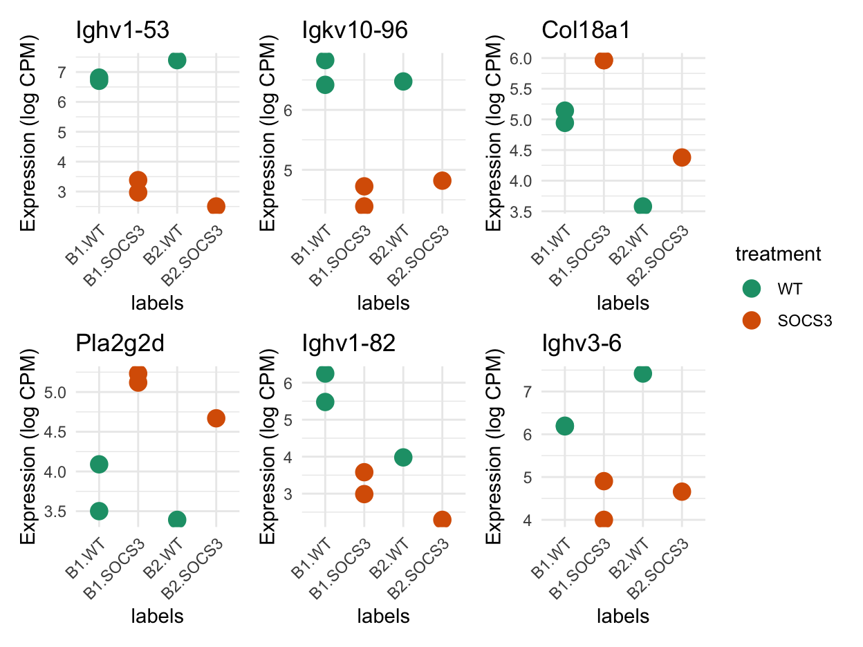

Show code

# Corresponds to:
head(de_table, n = 6)

          ensembl_transcript_id    ensembl_gene_id external_gene_name
Ighv1-53     ENSMUST00000103523 ENSMUSG00000093894           Ighv1-53
Igkv10-96    ENSMUST00000103328 ENSMUSG00000094420          Igkv10-96
Col18a1      ENSMUST00000081654 ENSMUSG00000001435            Col18a1
Pla2g2d      ENSMUST00000030528 ENSMUSG00000041202            Pla2g2d
Ighv1-82     ENSMUST00000196991 ENSMUSG00000095127           Ighv1-82
Ighv3-6      ENSMUST00000195124 ENSMUSG00000076672            Ighv3-6
          chromosome_name CHR    SYMBOL            ENSEMBL      logFC
Ighv1-53               12  12  Ighv1-53 ENSMUSG00000093894 -4.0124141
Igkv10-96               6   6 Igkv10-96 ENSMUSG00000094420 -1.9378250
Col18a1                10  10   Col18a1 ENSMUSG00000001435  0.8990599
Pla2g2d                 4   4   Pla2g2d ENSMUSG00000041202  1.3628040
Ighv1-82               12  12  Ighv1-82 ENSMUSG00000095127 -2.4104646
Ighv3-6                12  12   Ighv3-6 ENSMUSG00000076672 -2.1316224
           AveExpr          t      P.Value  adj.P.Val        B
Ighv1-53  4.959076 -15.353987 9.758266e-07 0.02124570 3.971764
Igkv10-96 5.608252 -11.850155 5.842989e-06 0.06360678 3.989723
Col18a1   4.994588   9.083638 3.517068e-05 0.24273285 2.661886
Pla2g2d   4.331964   8.659995 4.825114e-05 0.24273285 2.161525
Ighv1-82  4.091629  -8.069133 7.670576e-05 0.24273285 1.737427
Ighv3-6   5.559966  -7.996783 8.134194e-05 0.24273285 1.973738

The top 20 differentially expressed genes using voom are shown below.

Show code

# Top 20 genes
head(rownames(sorted_de), n=20)

 [1] "Ighv1-53"  "Igkv10-96" "Col18a1"   "Pla2g2d"   "Ighv1-82" 
 [6] "Ighv3-6"   "Igkv4-79"  "Ighv5-4"   "Kera"      "Ptx4"     
[11] "Serpina1d" "Atp6v0d2"  "Scx"       "Ighv2-2"   "Adamts3"  
[16] "Itk"       "St18"      "Spon2"     "Serpina1a" "Gm16867"

Treatment with edgeR::LRT method

Show code

design <- model.matrix(~ treatment + batch, data=dge$samples) 
dge <- estimateDisp(dge, design) 
fit <- glmFit(dge, design) 
lrt <- glmLRT(fit, coef = 2) 

# Find significant genes
de_results <- decideTests(lrt, adjust.method = "BH", p.value = 0.05)
summary(de_results)

       treatmentSOCS3
Down               59
NotSig          21691
Up                 22

Using glmLRT there are 59 genes which are downregulated in SOCS3, and 22 which are upregulated.

Show code

# MD plot
plotMD(lrt, status = de_results, values = c(-1, 1), col = c("blue", "red"), legend = "topright", main = "SOCS3 vs. WT")

Show code

de_table <- topTags(lrt, n = Inf)$table 
head(de_table)

          ensembl_transcript_id    ensembl_gene_id external_gene_name
Ighv1-53     ENSMUST00000103523 ENSMUSG00000093894           Ighv1-53
Serpina1d    ENSMUST00000078869 ENSMUSG00000071177          Serpina1d
Igkv4-79     ENSMUST00000103342 ENSMUSG00000076541           Igkv4-79
Igkv10-96    ENSMUST00000103328 ENSMUSG00000094420          Igkv10-96
Igkv9-124    ENSMUST00000196768 ENSMUSG00000096632          Igkv9-124
Ighv3-5      ENSMUST00000195619 ENSMUSG00000076670            Ighv3-5
          chromosome_name CHR    SYMBOL            ENSEMBL      logFC
Ighv1-53               12  12  Ighv1-53 ENSMUSG00000093894  -4.007728
Serpina1d              12  12 Serpina1d ENSMUSG00000071177  -9.776004
Igkv4-79                6   6  Igkv4-79 ENSMUSG00000076541 -10.546102
Igkv10-96               6   6 Igkv10-96 ENSMUSG00000094420  -1.934752
Igkv9-124               6   6 Igkv9-124 ENSMUSG00000096632  -6.219066
Ighv3-5                12  12   Ighv3-5 ENSMUSG00000076670  -7.575426
             logCPM        LR       PValue          FDR
Ighv1-53  6.0916737 143.76671 3.995733e-33 8.699510e-29
Serpina1d 2.5596776 128.73270 7.759510e-30 8.447003e-26
Igkv4-79  0.5236326 120.86874 4.082714e-28 2.962962e-24
Igkv10-96 5.9219024  85.87907 1.912824e-20 1.041150e-16
Igkv9-124 2.7873572  83.08807 7.847782e-20 3.417238e-16
Ighv3-5   0.6886644  52.57793 4.135092e-13 1.500487e-09

Show code

head(rownames(de_table), 20)

 [1] "Ighv1-53"  "Serpina1d" "Igkv4-79"  "Igkv10-96" "Igkv9-124"
 [6] "Ighv3-5"   "Ighv1-82"  "Ighv5-4"   "Ighv2-5"   "Ighv3-6"  
[11] "Pla2g2d"   "Igkv4-73"  "Igkv1-133" "Col18a1"   "Ighv1-25" 
[16] "Serpina1c" "Igkv3-5"   "Ighv1-63"  "Ighv1-55"  "Atp6v0d2"

Show code

# See the values of the DE for genes of interest
genes_of_interest <- c("Socs3", "Socs1", "Bcl3")

de_table[de_table$SYMBOL %in% genes_of_interest, ]

      ensembl_transcript_id    ensembl_gene_id external_gene_name
Socs1    ENSMUST00000229866 ENSMUSG00000038037              Socs1
Bcl3     ENSMUST00000135609 ENSMUSG00000053175               Bcl3
Socs3    ENSMUST00000054002 ENSMUSG00000053113              Socs3
      chromosome_name CHR SYMBOL            ENSEMBL      logFC
Socs1              16  16  Socs1 ENSMUSG00000038037 -0.1890986
Bcl3                7   7   Bcl3 ENSMUSG00000053175  0.1079021
Socs3              11  11  Socs3 ENSMUSG00000053113 -0.0964003
        logCPM        LR    PValue       FDR
Socs1 4.235511 0.8994515 0.3429288 0.9999886
Bcl3  5.572940 0.3537078 0.5520217 0.9999886
Socs3 8.363292 0.2785081 0.5976808 0.9999886

The LRT test also returns a number of Ig genes.

Plots of the most differentially expressed genes

Show code

top_genes <- head(rownames(de_table), n = 6)

selected_genes <- match(top_genes, rownames(dge))

df <- data.frame(
    y = t(lcpm[selected_genes, ]), 
    treatment = dge$samples$treatment, 
    batch = dge$samples$batch)

colnames(df)[1:length(top_genes)] <- rownames(dge)[selected_genes]

df$labels <- factor(paste0(df$batch, ".", df$treatment),
    levels=c("B1.WT", "B1.SOCS3", "B2.WT", "B2.SOCS3"))

plot_list <- list()
for (i in 1:length(top_genes)) {
    plot_list[[i]] <-
        ggplot(data = df, mapping = aes(x = labels, y = .data[[top_genes[i]]], group = labels, colour = treatment)) + 
            geom_point(size = 4) + 
            theme_minimal() + 
            theme(axis.text.x = element_text(angle = 45, hjust = 1)) + 
            ylab("Expression (log CPM)") + 
            scale_colour_manual(values = treatment_colours) +
            ggtitle(label = paste0(top_genes[i])
    )
}
patchwork::wrap_plots(plot_list, ncol = 3, guides = "collect")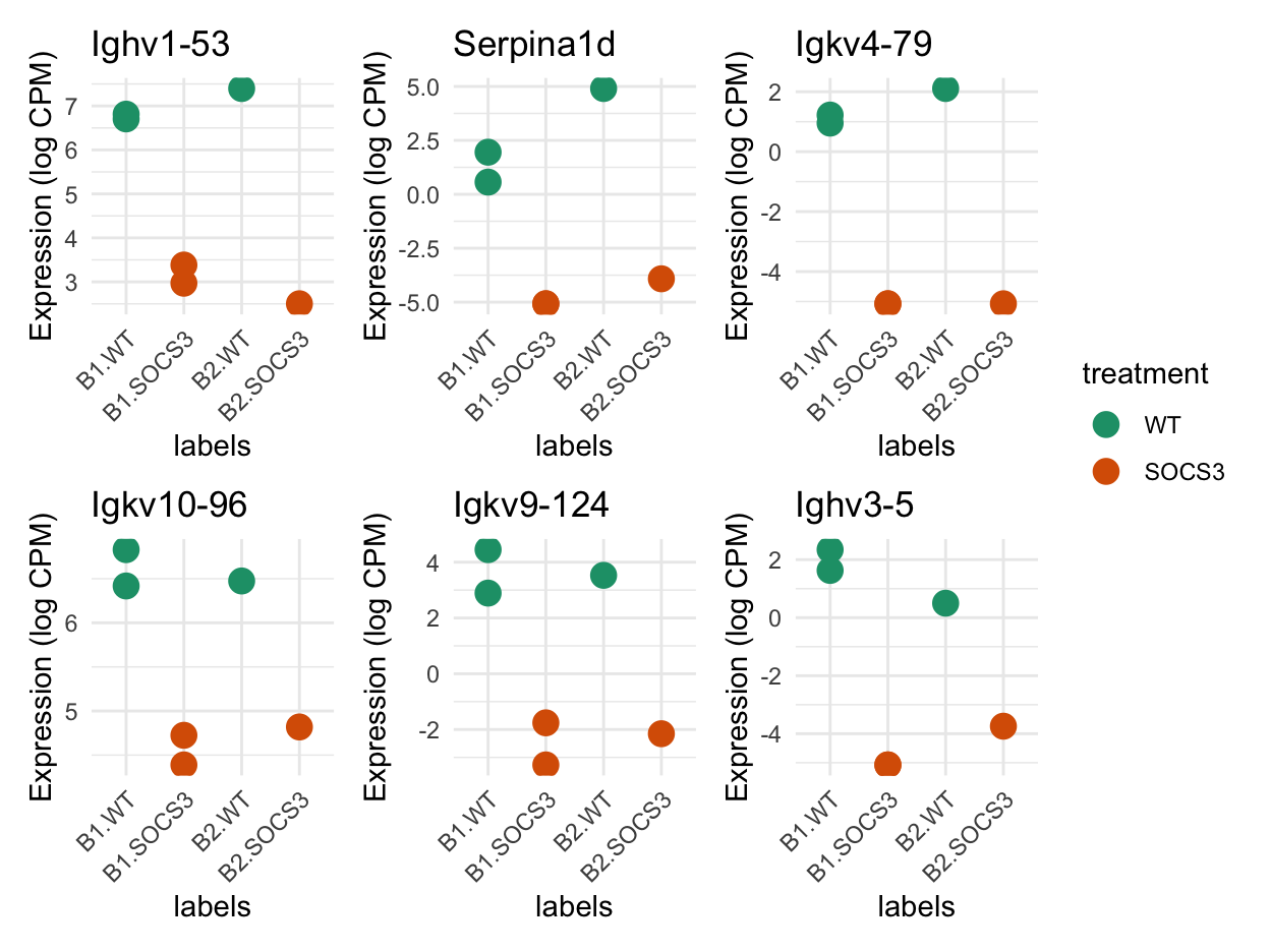

Show code

# Corresponds to:
head(de_table, n = 6)

          ensembl_transcript_id    ensembl_gene_id external_gene_name
Ighv1-53     ENSMUST00000103523 ENSMUSG00000093894           Ighv1-53
Serpina1d    ENSMUST00000078869 ENSMUSG00000071177          Serpina1d
Igkv4-79     ENSMUST00000103342 ENSMUSG00000076541           Igkv4-79
Igkv10-96    ENSMUST00000103328 ENSMUSG00000094420          Igkv10-96
Igkv9-124    ENSMUST00000196768 ENSMUSG00000096632          Igkv9-124
Ighv3-5      ENSMUST00000195619 ENSMUSG00000076670            Ighv3-5
          chromosome_name CHR    SYMBOL            ENSEMBL      logFC
Ighv1-53               12  12  Ighv1-53 ENSMUSG00000093894  -4.007728
Serpina1d              12  12 Serpina1d ENSMUSG00000071177  -9.776004
Igkv4-79                6   6  Igkv4-79 ENSMUSG00000076541 -10.546102
Igkv10-96               6   6 Igkv10-96 ENSMUSG00000094420  -1.934752
Igkv9-124               6   6 Igkv9-124 ENSMUSG00000096632  -6.219066
Ighv3-5                12  12   Ighv3-5 ENSMUSG00000076670  -7.575426
             logCPM        LR       PValue          FDR
Ighv1-53  6.0916737 143.76671 3.995733e-33 8.699510e-29
Serpina1d 2.5596776 128.73270 7.759510e-30 8.447003e-26
Igkv4-79  0.5236326 120.86874 4.082714e-28 2.962962e-24
Igkv10-96 5.9219024  85.87907 1.912824e-20 1.041150e-16
Igkv9-124 2.7873572  83.08807 7.847782e-20 3.417238e-16
Ighv3-5   0.6886644  52.57793 4.135092e-13 1.500487e-09

The heatmap below shows the top 50 genes with the highest differential expression. This is not the cleanest heatmap, with many genes which are only expressed highly in one of the three samples for a given treatment. In other words, many of the effects are driven by strong signals from one sample, rather than consistent differences across all three samples for a condition. The wild-type samples have higher expression of many Ig genes, while the Socs3 samples have higher expression of genes such as the mitochondrial gene mt-Co2 and the collagen gene Col18a1.

Show code

# Filter top 50 DE genes with FDR < 0.05
de_table_sig <- de_table[de_table$FDR < 0.05, ]
top50_genes <- rownames(head(de_table_sig, 50))

# Log2 CPM-normalized expression matrix
lcpm_top50 <- lcpm[top50_genes, ]

# Sample annotations: Treatment and Batch
annotation_col <- dge$samples[, c("treatment", "batch")]

# Z-score normalize rows (genes)
lcpm_scaled <- t(scale(t(lcpm_top50)))

# Plot heatmap
pheatmap(lcpm_scaled,
         annotation_col = annotation_col,
         annotation_colors = list(
             batch = batch_colours,
             treatment = treatment_colours),
         show_rownames = TRUE,
         show_colnames = FALSE,
         cluster_cols = TRUE,
         clustering_distance_rows = "euclidean",
         clustering_distance_cols = "euclidean",
         clustering_method = "complete",
         fontsize_row = 6,
         main = "Top DE genes for treatment using edgeR LRT \n (Uncorrected)")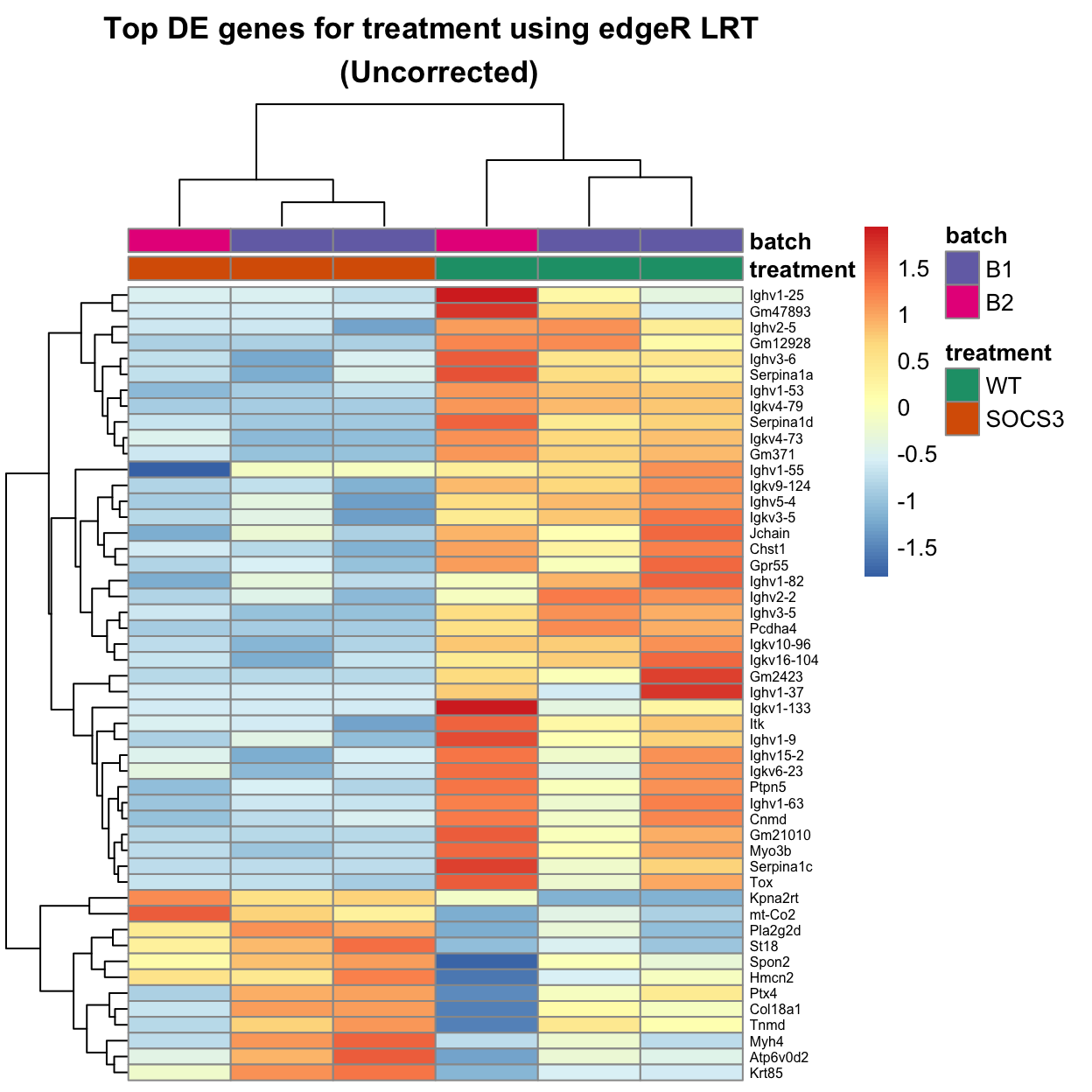

The heatmap below uses limma::removeBatchEffect to improve the visualisation. Note that the statistical test has not changed, this is just adjusting the values for plotting.

Show code

# Filter top 50 DE genes with FDR < 0.05
de_table_sig <- de_table[de_table$FDR < 0.05, ]
top50_genes <- rownames(head(de_table_sig, 50))


# Remove batch effect from logCPM for plotting
lcpm_corrected <- removeBatchEffect(lcpm, batch=dge$samples$batch)

# Log2 CPM-normalized expression matrix
lcpm_top50 <- lcpm_corrected[top50_genes, ]

# Sample annotations: Treatment and Batch
annotation_col <- dge$samples[, c("treatment", "batch")]

# Z-score normalize rows (genes)
lcpm_scaled <- t(scale(t(lcpm_top50)))

# Plot heatmap
pheatmap(lcpm_scaled,
         annotation_col = annotation_col,
         annotation_colors = list(
             batch = batch_colours,
             treatment = treatment_colours),
         show_rownames = TRUE,
         show_colnames = FALSE,
         cluster_cols = TRUE,
         clustering_distance_rows = "euclidean",
         clustering_distance_cols = "euclidean",
         clustering_method = "complete",
         fontsize_row = 6,
         main = "Top DE genes for treatment using edgeR LRT \n (Corrected)")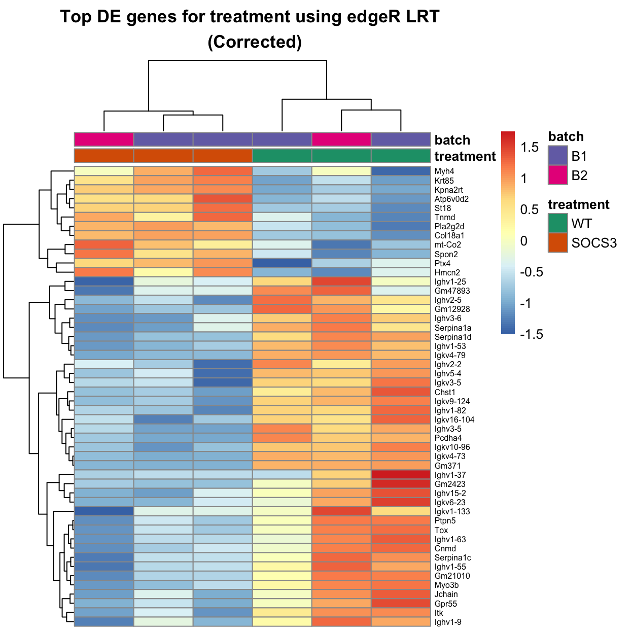

Show code

# The LRT de_results object is already sorted by FDR.

# Write to a file
dir.create(here("output/DEGs/kallisto_analysis"), recursive = TRUE)
write.table(de_table, file=here("output/DEGs/kallisto_analysis/kallisto_treatment_LRT.tsv"),
            sep="\t", quote=FALSE, row.names=FALSE)

A table of the differential expression results are saved in output/DEGs/kallisto_analysis/kallisto_treatment_LRT.tsv. The rows are sorted so the genes with the lowest FDR are at the top.

Batch with limma::voom method

There is a strong batch effect in this data set. In this section, I perform a DE test of just batch. This shows the genes that are upregulated in one batch but not the other, and are purely technical effects.

Show code

design <- model.matrix(~0+batch+treatment, data = dge$samples)

colnames(design) <- gsub("batch", "", colnames(design))
design

           B1 B2 treatmentSOCS3
WT_1_B2     0  1              0
SOCS3_1_B2  0  1              1
SOCS3_2_B1  1  0              1
SOCS3_3_B1  1  0              1
WT_2_B1     1  0              0
WT_3_B1     1  0              0
attr(,"assign")
[1] 1 1 2
attr(,"contrasts")
attr(,"contrasts")$batch
[1] "contr.treatment"

attr(,"contrasts")$treatment
[1] "contr.treatment"

Show code

contr.matrix <- makeContrasts(
   B2vsB1 = B2 - B1,
   levels = colnames(design))
contr.matrix

                Contrasts
Levels           B2vsB1
  B1                 -1
  B2                  1
  treatmentSOCS3      0

Show code

v <- voom(dge, design, plot=TRUE)

Show code

vfit <- lmFit(v, design)
vfit <- contrasts.fit(vfit, contrasts=contr.matrix)

efit <- eBayes(vfit)
plotSA(efit)

There are hundreds of genes in each direction which are significant when testing differences between batch 1 and batch 2.

Show code

tfit <- treat(vfit, lfc=0.1)
de_results <- decideTests(tfit)
summary(de_results)

       B2vsB1
Down      997
NotSig  20307
Up        468

Show code

# Sort the top table by adjusted P value
de_table <- topTable(tfit, number=Inf, sort.by="P")

head(rownames(de_table), n=20)

 [1] "Il1a"     "Rgs5"     "Tnf"      "Il1b"     "Rasgef1b" "Mfap4"   
 [7] "Cd14"     "Thbs4"    "Il10"     "Maff"     "Ccl4"     "Trim30b" 
[13] "Cd83"     "Sqstm1"   "Jcad"     "Sparcl1"  "Timp3"    "Col18a1" 
[19] "Clic4"    "Marcksl1"

Show code

sorted_de <- de_table[order(de_table$adj.P.Val), ]

# Write to a file
dir.create(here("output/DEGs/batch_effect"), recursive = TRUE)
write.table(sorted_de, file=here("output/DEGs/batch_effect/kallisto_batch_voom.tsv"),
            sep="\t", quote=FALSE, row.names=FALSE)

Show code

# Filter DE genes with FDR < 0.05
de_table_sig <- de_table[de_table$adj.P.Val < 0.05, ]

# Select top 50 DE genes by smallest FDR
top50_genes <- head(rownames(de_table_sig), 50)

# Use voom-transformed expression matrix
expr_mat <- v$E[top50_genes, ]

# Sample annotations
annotation_col <- dge$samples[, c("batch", "treatment")]

# Z-score normalize rows (genes)
lcpm_scaled <- t(scale(t(expr_mat)))

# Plot heatmap
pheatmap(lcpm_scaled,
         annotation_col = annotation_col,
         annotation_colors = list(
             batch = batch_colours,
             treatment = treatment_colours),
         show_rownames = TRUE,
         show_colnames = FALSE,
         cluster_cols = FALSE,
         clustering_distance_rows = "euclidean",
         clustering_distance_cols = "euclidean",
         clustering_method = "complete",
         fontsize_row = 6,
         main = "Top DE genes for batch using voom")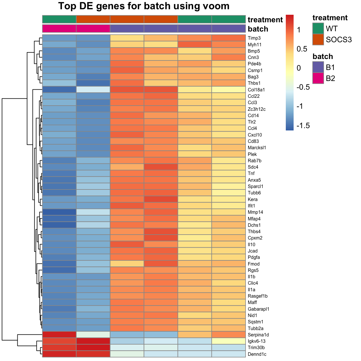

DE if we remove WT_2_B1

This analysis uses the limma::voom method. We remove the problematic sample in the batch 1 group and reprocess the data. MDS plots of the data without this sample are shown below.

Show code

dge2 <- dge[, dge$samples$group != "WT_2_B1"]

lcpm2 <- edgeR::cpm(dge2, log = TRUE)

par(mfrow = c(2,2))
plotMDS(lcpm2, labels=colnames(lcpm2), col=group_colours[colnames(lcpm2)])
title(main="A. Sample groups")

plotMDS(lcpm2, labels=dge2$samples$treatment, col=treatment_colours[dge2$samples$treatment])
title(main="B. Treatment")

plotMDS(lcpm2, labels=dge2$samples$batch, col=batch_colours[dge2$samples$batch])
title(main="C. Batch")

# MDS plot with library size
libsizes2 <- dge2$samples$lib.size

# Create a viridis color function
color_func <- scales::col_numeric(viridis::viridis(100), domain = range(libsizes2))

# Assign colors according to library sizes
point_colors2 <- color_func(libsizes2)

plotMDS(lcpm2, labels=NULL, pch = 16, cex = 4, col=point_colors2)
title(main="D. Library Size")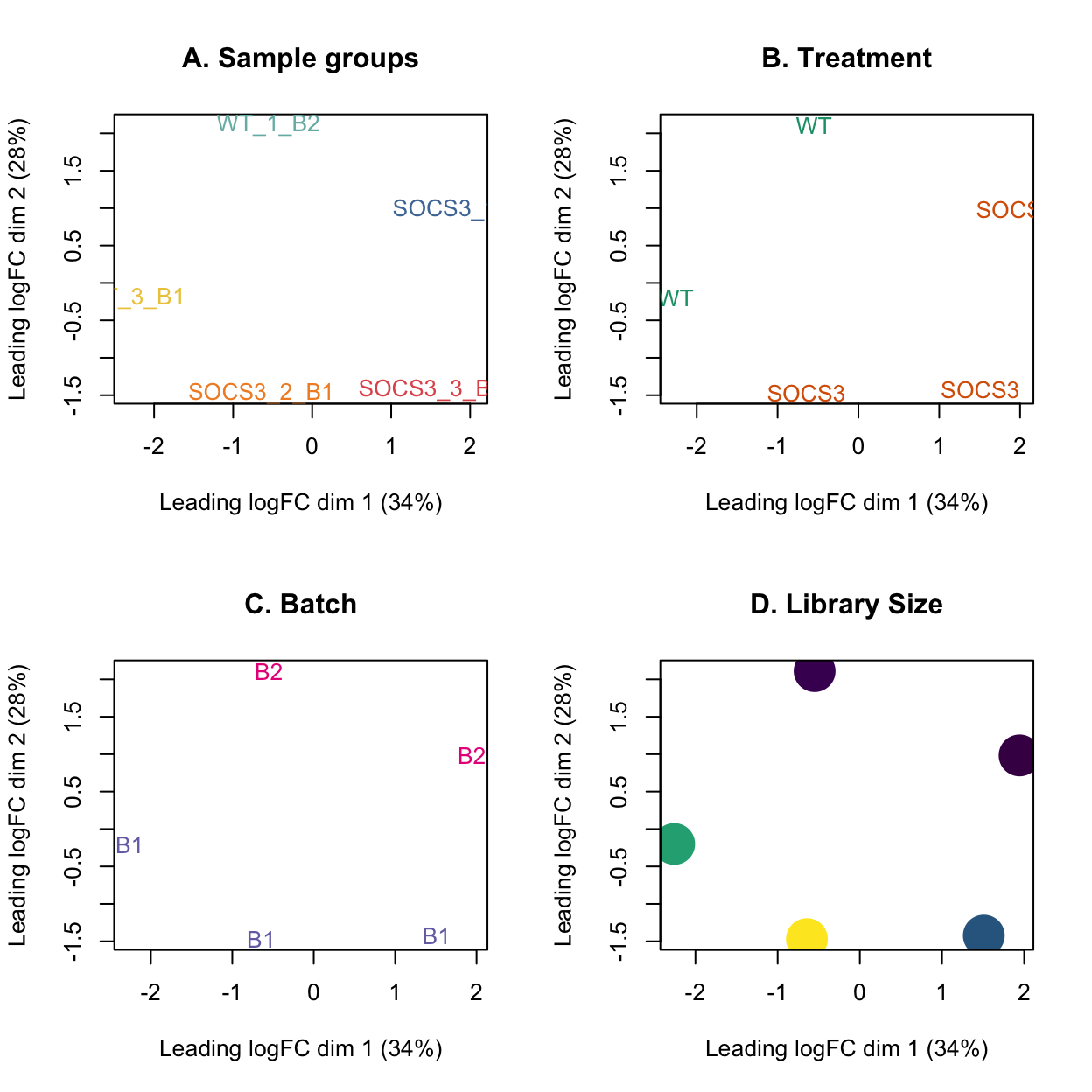

Show code

design <- model.matrix(~0+treatment+batch, data = dge2$samples)

colnames(design) <- gsub("treatment|batch", "", colnames(design))

contr.matrix <- makeContrasts(
   SOCS3vsWT = SOCS3 - WT,
   levels = colnames(design))
contr.matrix

       Contrasts
Levels  SOCS3vsWT
  WT           -1
  SOCS3         1
  B2            0

Show code

v <- voom(dge2, design, plot=TRUE)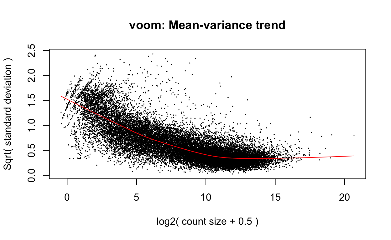

Show code

vfit <- lmFit(v, design)
vfit <- contrasts.fit(vfit, contrasts=contr.matrix)

efit <- eBayes(vfit)
plotSA(efit)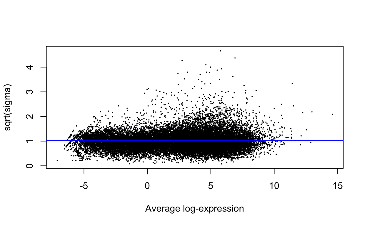

Show code

tfit <- treat(vfit, lfc=0.1)
de_results <- decideTests(tfit)
summary(de_results)

       SOCS3vsWT
Down          11
NotSig     21761
Up             0

There are 11 genes which are more highly expressed in the controls. The “Ig” genes and “Jchain” are related to B-cells and plasma cells.

Show code

# Sort the top table by adjusted P value
sorted_de <- topTable(tfit, number=Inf, sort.by="P")
sorted_de <- sorted_de[order(sorted_de$adj.P.Val), ]

head(rownames(sorted_de), n=20)

 [1] "Igkv6-23"  "Ighv1-53"  "Igkv6-15"  "Igkv10-96" "Ighv1-55" 
 [6] "Jchain"    "Tox"       "Ighv1-82"  "Igkv9-124" "Igha"     
[11] "Gpr55"     "Ighv1-72"  "Cnmd"      "Ighv1-58"  "Pla2g2d"  
[16] "Ighv5-4"   "Serpina1d" "Bcl11b"    "Tnfsf8"    "Ptpn5"

Show code

# Write to a file
write.table(sorted_de, file=here("output/DEGs/kallisto_analysis/kallisto_5samples_treatment_voom.tsv"),
            sep="\t", quote=FALSE, row.names=FALSE)

DE with random treatment labels

If we randomly permute the treatment labels, i.e., intentionally mess up our data, what does the LRT test look like? This section uses limma::voom().

Show code

set.seed(123)

Show code

# Copy the object
dge_ <- dge

# Shuffle treatment labels
dge_$samples$treatment <- sample(dge_$samples$treatment)

design_ <- model.matrix(~ treatment + batch, data = dge_$samples) 
dge_ <- estimateDisp(dge_, design_) 
fit_ <- glmFit(dge_, design_) 
lrt_ <- glmLRT(fit_, coef = 2) 

# Find significant genes
de_results_ <- decideTests(lrt_, adjust.method = "BH", p.value = 0.05)

There are far fewer DE genes in this case, which shows that our signal above is likely to be real.

Show code

summary(de_results_)

       treatmentSOCS3
Down                4
NotSig          21767
Up                  1

Show code

de_table_ <- topTags(lrt_, n = Inf)$table 
head(de_table_, n=20)

          ensembl_transcript_id    ensembl_gene_id external_gene_name
Gm2007       ENSMUST00000177981 ENSMUSG00000094932             Gm2007
Gm15229      ENSMUST00000146636 ENSMUSG00000085880            Gm15229
Foxc1        ENSMUST00000062292 ENSMUSG00000050295              Foxc1
Ighv1-75     ENSMUST00000103544 ENSMUSG00000096020           Ighv1-75
Ighv8-5      ENSMUST00000194257 ENSMUSG00000102364            Ighv8-5
Potefam3a    ENSMUST00000084046 ENSMUSG00000074449          Potefam3a
Myh4         ENSMUST00000018632 ENSMUSG00000057003               Myh4
Ighv3-8      ENSMUST00000103483 ENSMUSG00000076674            Ighv3-8
Kcnk18       ENSMUST00000065204 ENSMUSG00000040901             Kcnk18
Lum          ENSMUST00000038160 ENSMUSG00000036446                Lum
Mroh4        ENSMUST00000137963 ENSMUSG00000022603              Mroh4
Bglap        ENSMUST00000076048 ENSMUSG00000074483              Bglap
Dsc3         ENSMUST00000115848 ENSMUSG00000059898               Dsc3
Alpl         ENSMUST00000030551 ENSMUSG00000028766               Alpl
Stmnd1       ENSMUST00000076622 ENSMUSG00000063529             Stmnd1
Enpp3        ENSMUST00000020169 ENSMUSG00000019989              Enpp3
Kpna2-ps     ENSMUST00000120025 ENSMUSG00000083672           Kpna2-ps
Gm12226      ENSMUST00000144172 ENSMUSG00000078151            Gm12226
Igkv5-39     ENSMUST00000103370 ENSMUSG00000076569           Igkv5-39
Ighv3-4      ENSMUST00000193408 ENSMUSG00000103939            Ighv3-4
          chromosome_name CHR    SYMBOL            ENSEMBL      logFC
Gm2007                  2   2    Gm2007 ENSMUSG00000094932 -9.7052087
Gm15229                 X   X   Gm15229 ENSMUSG00000085880  7.2062234
Foxc1                  13  13     Foxc1 ENSMUSG00000050295 -0.8019353
Ighv1-75               12  12  Ighv1-75 ENSMUSG00000096020 -3.7895471
Ighv8-5                12  12   Ighv8-5 ENSMUSG00000102364 -6.9525198
Potefam3a               8   8 Potefam3a ENSMUSG00000074449  6.8569197
Myh4                   11  11      Myh4 ENSMUSG00000057003  5.1951482
Ighv3-8                12  12   Ighv3-8 ENSMUSG00000076674 -4.6346699
Kcnk18                 19  19    Kcnk18 ENSMUSG00000040901 -6.3120558
Lum                    10  10       Lum ENSMUSG00000036446 -1.0588937
Mroh4                  15  15     Mroh4 ENSMUSG00000022603  6.3786357
Bglap                   3   3     Bglap ENSMUSG00000074483 -0.8781689
Dsc3                   18  18      Dsc3 ENSMUSG00000059898  6.4164619
Alpl                    4   4      Alpl ENSMUSG00000028766 -0.6351976
Stmnd1                 13  13    Stmnd1 ENSMUSG00000063529  6.2499584
Enpp3                  10  10     Enpp3 ENSMUSG00000019989 -1.0425094
Kpna2-ps               17  17  Kpna2-ps ENSMUSG00000083672  7.2980602
Gm12226                11  11   Gm12226 ENSMUSG00000078151 -5.0751752
Igkv5-39                6   6  Igkv5-39 ENSMUSG00000076569 -2.4204263
Ighv3-4                12  12   Ighv3-4 ENSMUSG00000103939  7.9808127
              logCPM       LR       PValue          FDR
Gm2007    -0.2703938 66.79157 3.017859e-16 6.570482e-12
Gm15229   -2.5835771 23.12997 1.514125e-06 1.132512e-02
Foxc1      6.0478221 23.07195 1.560508e-06 1.132512e-02
Ighv1-75   2.6232300 21.42692 3.675736e-06 1.602908e-02
Ighv8-5   -2.8281855 21.42411 3.681123e-06 1.602908e-02
Potefam3a -2.7869402 18.82521 1.432611e-05 5.198469e-02
Myh4      -1.3660936 18.17569 2.014340e-05 5.894397e-02
Ighv3-8    3.1170949 18.03759 2.165863e-05 5.894397e-02
Kcnk18    -3.3130169 17.20649 3.352893e-05 8.053663e-02
Lum        8.6332902 16.89493 3.950702e-05 8.053663e-02
Mroh4     -3.2180534 16.83308 4.081556e-05 8.053663e-02
Bglap      6.0856786 16.66580 4.457736e-05 8.053663e-02
Dsc3      -3.1228978 16.52203 4.808820e-05 8.053663e-02
Alpl       7.3573092 16.04277 6.192748e-05 8.109438e-02
Stmnd1    -3.2621636 16.01031 6.299860e-05 8.109438e-02
Enpp3      3.6304868 15.99791 6.341246e-05 8.109438e-02
Kpna2-ps  -2.3413436 15.94451 6.522661e-05 8.109438e-02
Gm12226   -2.2529186 15.89247 6.704478e-05 8.109438e-02
Igkv5-39   5.0866049 15.30925 9.126871e-05 9.706066e-02
Ighv3-4   -1.6262437 15.28273 9.255876e-05 9.706066e-02

Concluding remarks

The output/DEGs/ directory contains CSV files summarising the differential expression results. The following are available on request:

Full CSV tables of any data presented.
PDF/PNG files of any static plots.

Analysis of the Socs3 knockout data with kallisto alignment.

Introduction

Setting up the data

Reading in count data

Kallisto mapping information

Organising sample information

Organising gene annotations

Pre-processing

Quality control

Library size

Number of expressed features

Proportion of mitochondrial genes

Normalisation

Visualising the data

Comparing batches for genes of interest

Differential Expression Analyses

Treatment with limma::voom method

Plots of the most differentially expressed genes

Treatment with edgeR::LRT method

Plots of the most differentially expressed genes

Batch with limma::voom method

DE if we remove WT_2_B1

DE with random treatment labels

Concluding remarks