Introduction

This analysis is based on the guide “RNA-seq analysis is easy as 1-2-3 with limma, Glimma and edgeR” (Law et al. 2018), see https://pmc.ncbi.nlm.nih.gov/articles/PMC4937821/.

Show code

# Load required libraries for the document 
library(limma) 
library(edgeR) 
library(RColorBrewer) 
library(ggplot2) 
library(gridExtra) 
library(here)
library(dplyr)
library(ggplot2)
library(patchwork)
# BiocManager::install("Mus.musculus")
library(Mus.musculus)
library(RColorBrewer)

Setting up the data

This analysis uses the filtered_output_3 data. The pre-processing included cutadapt for trimming adapter sequences, trimmomatic, and hisat2 for alignment.

Reading in count data

Show code

# Read in data
counts <- read.csv(here("data/old_counts/filtered_output_3_combined_counts.csv"), header=TRUE) 
rownames(counts) <- counts$gene 
counts <- counts[, -1]   

# Remove everything before the full stop
colnames(counts) <- factor(gsub("filtered_output2_|260_|985_|Tube._", "", colnames(counts)))
group <- factor(colnames(counts))

dge <- DGEList(counts)
class(dge)

[1] "DGEList"
attr(,"package")
[1] "edgeR"

Organising sample information

Show code

# Better to get the batch from the colnames also
batch <- gsub(".+_", "", group)
batch <- factor(gsub("B", "Batch", batch))

# Replace uppercase with lowercase
group <- factor(group)
# Treatment labels SOCS3 or WT
treatment <- factor(gsub("_.+", "", group))

# Put sample information info DGEList object
dge$samples$group <- group
dge$samples$batch <- batch
dge$samples$treatment <- treatment

# Check that everything is consistent here
table(group, treatment)

            treatment
group        SOCS3 WT
  SOCS3_1_B2     1  0
  SOCS3_2_B1     1  0
  SOCS3_3_B1     1  0
  WT_1_B2        0  1
  WT_2_B1        0  1
  WT_3_B1        0  1

Show code

table(group, batch)

            batch
group        Batch1 Batch2
  SOCS3_1_B2      0      1
  SOCS3_2_B1      1      0
  SOCS3_3_B1      1      0
  WT_1_B2         0      1
  WT_2_B1         1      0
  WT_3_B1         1      0

Show code

dge$samples

                group lib.size norm.factors  batch treatment
WT_1_B2       WT_1_B2 10384129            1 Batch2        WT
SOCS3_1_B2 SOCS3_1_B2 11483449            1 Batch2     SOCS3
SOCS3_2_B1 SOCS3_2_B1 12461036            1 Batch1     SOCS3
SOCS3_3_B1 SOCS3_3_B1 10799372            1 Batch1     SOCS3
WT_2_B1       WT_2_B1  9901505            1 Batch1        WT
WT_3_B1       WT_3_B1 10645117            1 Batch1        WT

Show code

# Remove group, treatment and batch. These should only be accessed from dge!!!
rm(group, batch, treatment)

Organising gene annotations

Show code

geneid <- rownames(dge)

# We have Ensembl ID's
gene_map <- AnnotationDbi::select(Mus.musculus, keys=geneid, columns=c("SYMBOL", "TXCHROM"), 
                keytype="ENSEMBL")

# Investigate duplicate gene IDs

# There are 63 duplicate IDs, for these use their Ensembl ID ... or just remove them?
# Code to remove them:
# table(duplicated(gene_map$ENSEMBL))
gene_map$SYMBOL[duplicated(gene_map$ENSEMBL)] <- gene_map$ENSEMBL[duplicated(gene_map$ENSEMBL)]

# For NA symbols, use the ensembl gene id
gene_map$SYMBOL <- ifelse(is.na(gene_map$SYMBOL), gene_map$ENSEMBL, gene_map$SYMBOL) 
dge$genes <- gene_map[match(rownames(dge), gene_map$ENSEMBL), ]

# head(dge$genes)

# Check that the gene information matches the ordering of the count matrix
stopifnot(identical(rownames(dge), dge$genes$ENSEMBL))

Pre-processing

Filter low quality genes

Show code

# Transform from raw scale
cpm <- edgeR::cpm(dge)
lcpm <- edgeR::cpm(dge, log = TRUE)

The table below shows the number of non-zero counts there are for the 21700 genes in the data currently. There are 4201 genes which aren’t expressed in any samples, which will be removed from the data set.

Show code

table(rowSums(dge$counts > 0))


    0     1     2     3     4     5     6 
 4201  1452  1035   868   896  1119 12129

Show code

keep.exprs <- filterByExpr(dge, group=dge$samples$group)
dge <- dge[keep.exprs,, keep.lib.sizes=FALSE]


# sum(keep.exprs == FALSE)
# rowSums(dge$counts == 0)

There are 13579 genes remaining, and 8121 genes were removed.

In the raw data, there is a spike of lowly expressed genes. These are removed using the filterByExpr function.

Show code

# Figure 1: Density of the raw post filtered data

# M is the mean, L is the median
L <- mean(dge$samples$lib.size) * 1e-6
M <- median(dge$samples$lib.size) * 1e-6

lcpm.cutoff <- log2(10/M + 2/L)
nsamples <- ncol(dge)
col <- brewer.pal(nsamples, "Paired")
par(mfrow=c(1,2))
plot(density(lcpm[,1]), col=col[1], lwd=2, ylim=c(0,0.26), las=2, main="", xlab="")
title(main="A. Raw data", xlab="Log-cpm")
abline(v=lcpm.cutoff, lty=3)
for (i in 2:nsamples){
  den <- density(lcpm[,i])
  lines(den$x, den$y, col=col[i], lwd=2)
}
legend("topright", as.character(dge$samples$group), text.col=col, bty="n")
lcpm <- edgeR::cpm(dge, log=TRUE)
plot(density(lcpm[,1]), col=col[1], lwd=2, ylim=c(0,0.26), las=2, main="", xlab="")
title(main="B. Filtered data", xlab="Log-cpm")
abline(v=lcpm.cutoff, lty=3)
for (i in 2:nsamples){
  den <- density(lcpm[,i])
  lines(den$x, den$y, col=col[i], lwd=2)
}
legend("topright", as.character(dge$samples$group), text.col=col, bty="n")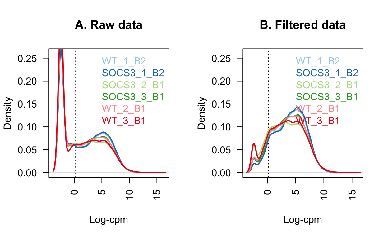

Quality control

Show code

# Set colours for this data set
group_colours <- setNames(
    ggthemes::tableau_color_pal("Tableau 10")(6), 
    levels(dge$samples$group))

batch_colours <- setNames(
    brewer.pal(8, "Dark2")[3:4], 
    levels(dge$samples$batch))

treatment_colours <- setNames(
    brewer.pal(8, "Dark2")[1:2], 
    levels(dge$samples$treatment))

Library size

The barcharts below show the library sizes for each sample, coloured by sample, batch and treatment.

Show code

# this factor ordering for group is helpful for QC, as it puts everything from 
# the same batch next to each other. 
dge$samples$group <- factor(dge$samples$group,
    levels = c("WT_2_B1", "WT_3_B1", "SOCS3_2_B1", "SOCS3_3_B1", "WT_1_B2", "SOCS3_1_B2"))

p1 <- ggplot(data = dge$samples, mapping = aes(y = group, x = lib.size, fill = group)) + 
    geom_col() +
    scale_fill_manual(values = group_colours) +
    scale_y_discrete(limits = rev(levels(dge$samples$group))) +
    theme_minimal()
p2 <- ggplot(data = dge$samples, mapping = aes(y = group, x = lib.size, fill = batch)) + 
    geom_col() +
    scale_fill_manual(values = batch_colours) +
    scale_y_discrete(limits = rev(levels(dge$samples$group))) +
    theme_minimal()
p3 <- ggplot(data = dge$samples, mapping = aes(y = group, x = lib.size, fill = treatment)) + 
    geom_col() +
    scale_fill_manual(values = treatment_colours) + 
    scale_y_discrete(limits = rev(levels(dge$samples$group))) +
    theme_minimal()
(p1 / p2 / p3) + plot_layout(guides = "collect")

Number of expressed features

Expressed features are defined as those with at least one count in a sample. There is a similar number of expressed features in each sample. Note however that 13,000 is quite low and the usual amount would be closer to 20,000 genes. This can be explained by the mapping strategy and pre-processing steps used for this data.

Show code

dge$samples$nFeatures <- apply(dge$counts, MARGIN = 2, FUN = function(x) {sum(x > 0)})

dge$samples |>
    dplyr::select(group, nFeatures) |>
    knitr::kable()

	group	nFeatures
WT_1_B2	WT_1_B2	13358
SOCS3_1_B2	SOCS3_1_B2	13368
SOCS3_2_B1	SOCS3_2_B1	12831
SOCS3_3_B1	SOCS3_3_B1	13213
WT_2_B1	WT_2_B1	13193
WT_3_B1	WT_3_B1	12746

Proportion of mitochondrial genes

There are no mitochondrial genes in this count matrix.

Show code

table(dge$genes$TXCHROM)


                chr1                chr10                chr11 
                 836                  644                 1145 
               chr12                chr13                chr14 
                 462                  436                  420 
               chr15                chr16                chr17 
                 559                  399                  663 
               chr18                chr19                 chr2 
                 343                  512                 1054 
                chr3                 chr4 chr4_JH584294_random 
                 578                  902                    1 
                chr5                 chr6                 chr7 
                 815                  755                 1043 
                chr8                 chr9                 chrX 
                 632                  758                  333

Normalisation

The impact of normalisation is subtle. Most notably, the third quantiles have been brought into alignment.

Show code

dge_raw <- dge
dge <- calcNormFactors(dge, method = "TMM")

The library sizes for the samples are listed in the table below. This is the sum of counts across every gene for that sample.

Show code

# Library sizes
dge_raw$sample |> 
    dplyr::select(lib.size) |>
    knitr::kable()

	lib.size
WT_1_B2	10377317
SOCS3_1_B2	11475960
SOCS3_2_B1	12456805
SOCS3_3_B1	10793544
WT_2_B1	9896663
WT_3_B1	10641492

Show code

# log-cpm in appropriate order for plot
# NOTE: NEVER USE WITH dge$samples!!! For plotting only!!
lcpm_raw_plot <- edgeR::cpm(dge_raw, log=TRUE)[, levels(dge_raw$samples$group)]
lcpm_plot <- edgeR::cpm(dge, log = TRUE)[, levels(dge$samples$group)]

# y-limit for plot 
ylims <- range(c(lcpm_raw_plot, lcpm_plot))
par(mfrow=c(1,2))

boxplot(lcpm_raw_plot, las=2, col=col, main="", )
title(main="A. Example: Unnormalised data", ylab="Log-cpm")

boxplot(lcpm_plot, las=2, col=col, main="")
title(main="B. Example: Normalised data", ylab="Log-cpm")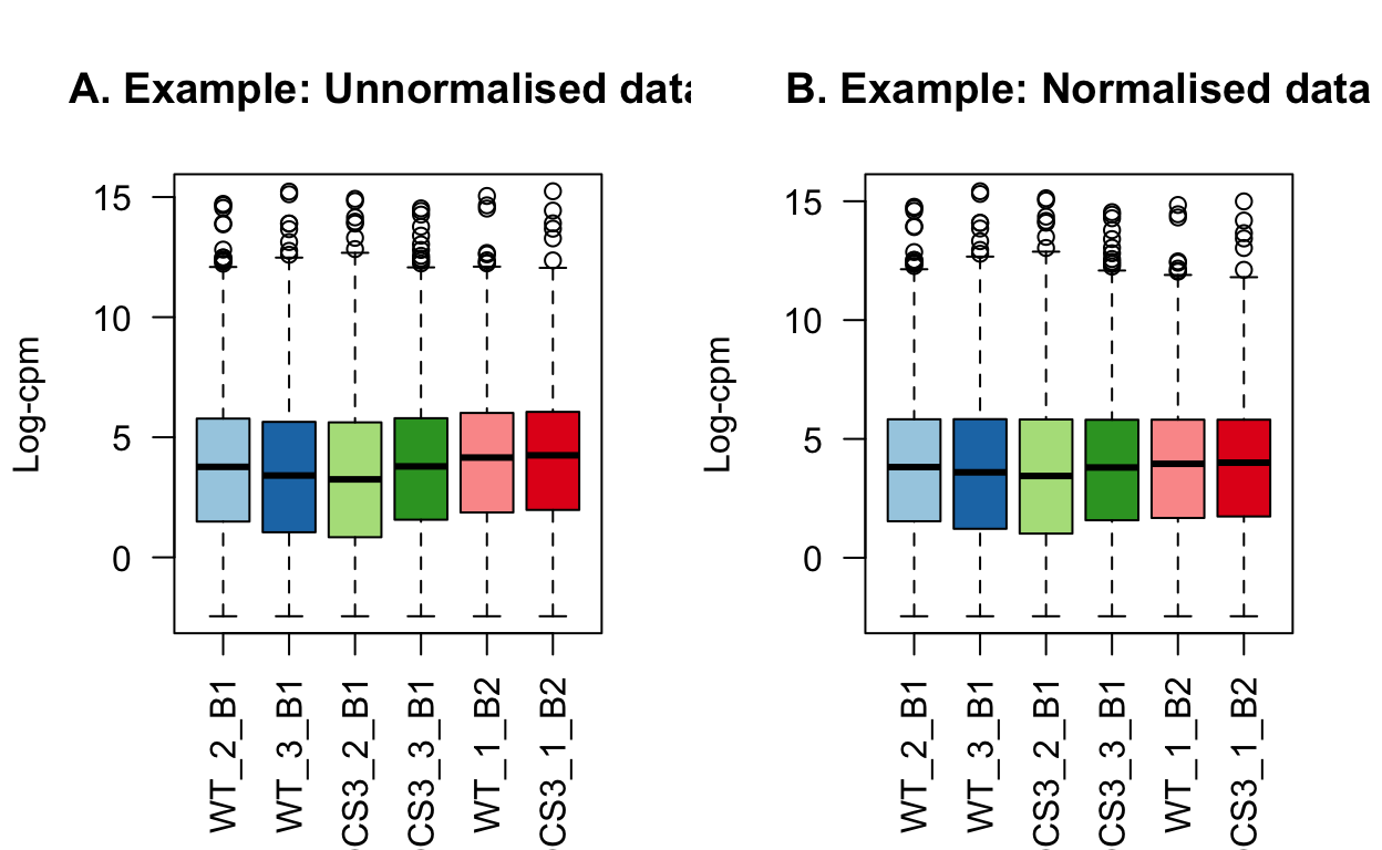

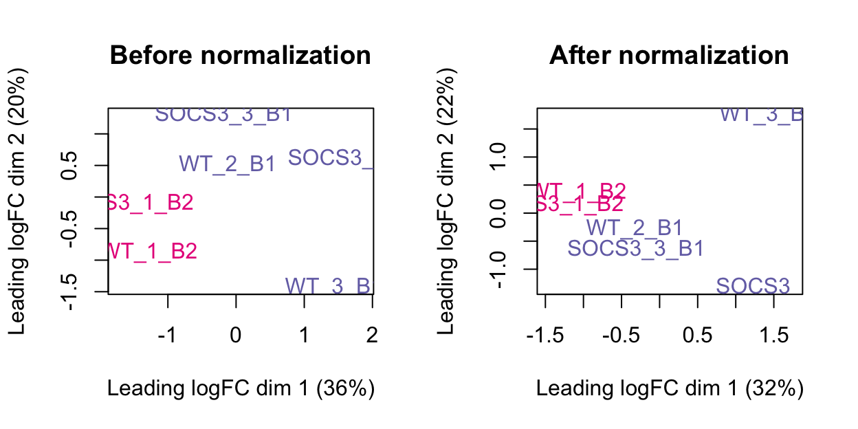
The plots below show the MDS plot before and after normalisation. This has a more obvious difference than the boxplot above.

Show code

par(mfrow = c(1,2))
plotMDS(dge_raw, main="Before normalization", col=batch_colours[dge_raw$samples$batch])
plotMDS(dge, main="After normalization", col=batch_colours[dge$samples$batch])

After normalising the data, we need to evaluate the log counts again.

Show code

cpm <- edgeR::cpm(dge)
lcpm <- edgeR::cpm(dge, log=TRUE)

Visualising the data

A useful tool to visualise RNA-seq data is the multi-dimensional scaling (MDS) plot. This plot can show us which samples are more similar to each other, and can help to identify outlying or low quality samples. The first dimension captures the largest amount of information about the data, while the second dimension captures the next biggest proportion of variation.

Things to look out for in this plot are:

Samples should cluster within the primary condition of interest, i.e., treatment.
Technical replicates should lie very close to each other.
The first dimension should explain treatment, and the second should explain batch.

The MDS plot below shows that the first dimension can be explained by batch (32% variation). The second dimension shows some separation by treatment and library size.

As the technical replicates have not clustered together, we cannot get DE for this data.

Show code

# NOTE: Even though it might seem like more typing, it is much better to use
#   dge$samples$group than group. 
#   It is very easy to have inconsistencies with labelling if not using the dge
#   object every time. 
par(mfrow = c(2,2))
plotMDS(lcpm, labels=dge$samples$group, col=group_colours[dge$samples$group])
title(main="A. Sample groups")

plotMDS(lcpm, labels=dge$samples$treatment, col=treatment_colours[dge$samples$treatment])
title(main="B. Treatment")

plotMDS(lcpm, labels=dge$samples$batch, col=batch_colours[dge$samples$batch])
title(main="C. Batch")

# MDS plot with library size
libsizes <- dge$samples$lib.size

# Create a viridis color function
color_func <- scales::col_numeric(viridis::viridis(100), domain = range(libsizes))

# Assign colors according to library sizes
point_colors <- color_func(libsizes)

plotMDS(lcpm, labels=NULL, pch = 16, cex = 4, col=point_colors)
title(main="D. Library Size")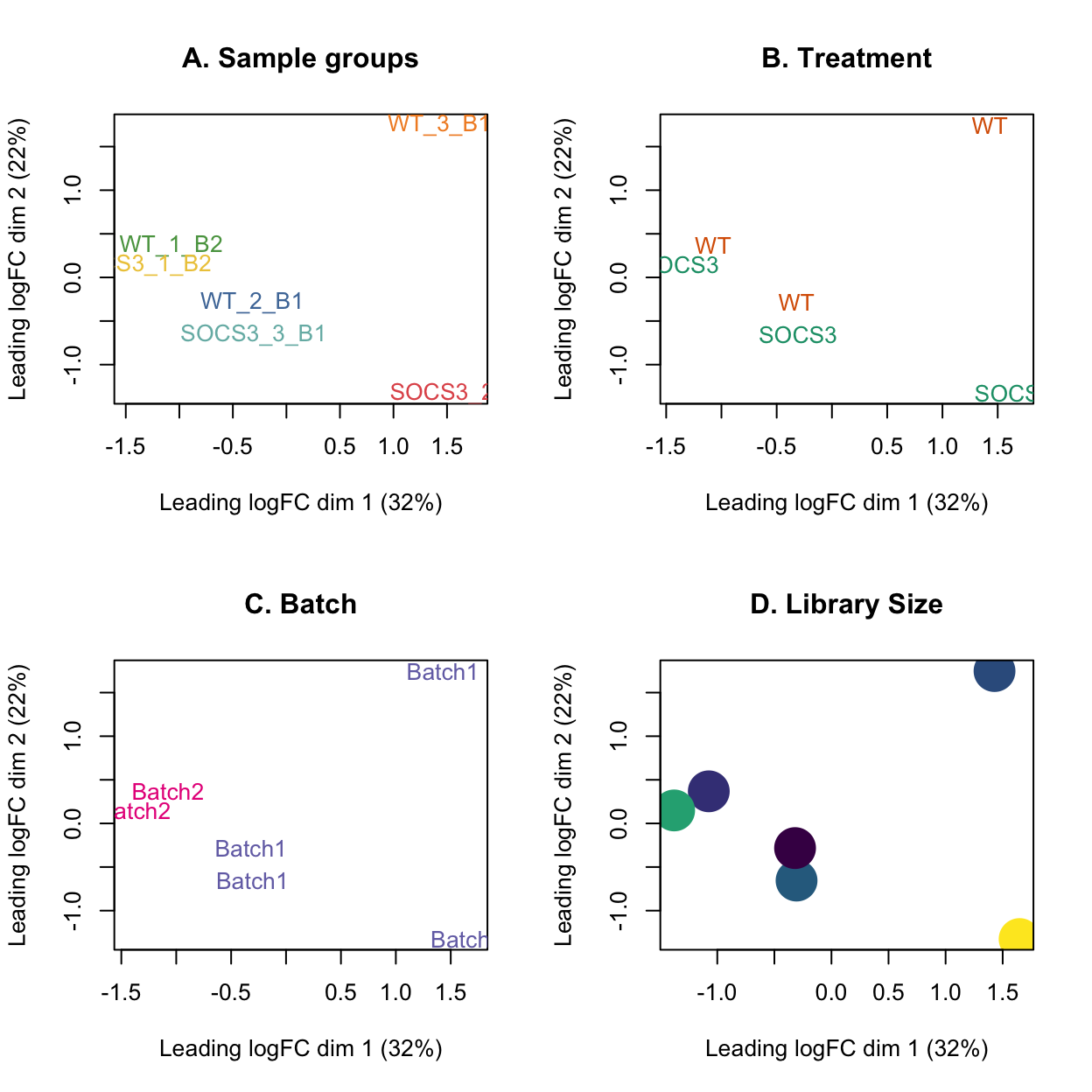

Plots showing genes of interest on MDS plot.

Show code

par(mfrow = c(2,2))

# Plot 3: Treatments 
plotMDS(lcpm, labels=dge$samples$treatment, col=treatment_colours[dge$samples$treatment])
title(main="C. Treatment") 


genes_of_interest <- c("Socs3", "Socs1", "Bcl3")

# Plot 5: Socs gene. 
gene_name <- genes_of_interest[1]
gene_expression <- lcpm[grep(gene_name, dge$genes$SYMBOL), ]

# Create a viridis color function
color_func <- scales::col_numeric(viridis::viridis(100), domain = range(gene_expression))

# Assign colors according to library sizes
point_colors <- color_func(gene_expression)

plotMDS(lcpm, labels=NULL, pch = 16, cex = 4, col=point_colors)
title(main=paste0(gene_name, " Expression (log CPM)")) 


gene_name <- genes_of_interest[2]
gene_expression <- lcpm[grep(gene_name, dge$genes$SYMBOL), ]

# Create a viridis color function
color_func <- scales::col_numeric(viridis::viridis(100), domain = range(gene_expression))

# Assign colors according to library sizes
point_colors <- color_func(gene_expression)

plotMDS(lcpm, labels=NULL, pch = 16, cex = 4, col=point_colors)
title(main=paste0(gene_name, " Expression (log CPM)")) 


gene_name <- genes_of_interest[3]
gene_expression <- lcpm[grep(gene_name, dge$genes$SYMBOL), ]

# Create a viridis color function
color_func <- scales::col_numeric(viridis::viridis(100), domain = range(gene_expression))

# Assign colors according to library sizes
point_colors <- color_func(gene_expression)

plotMDS(lcpm, labels=NULL, pch = 16, cex = 4, col=point_colors)
title(main=paste0(gene_name, " Expression (log CPM)"))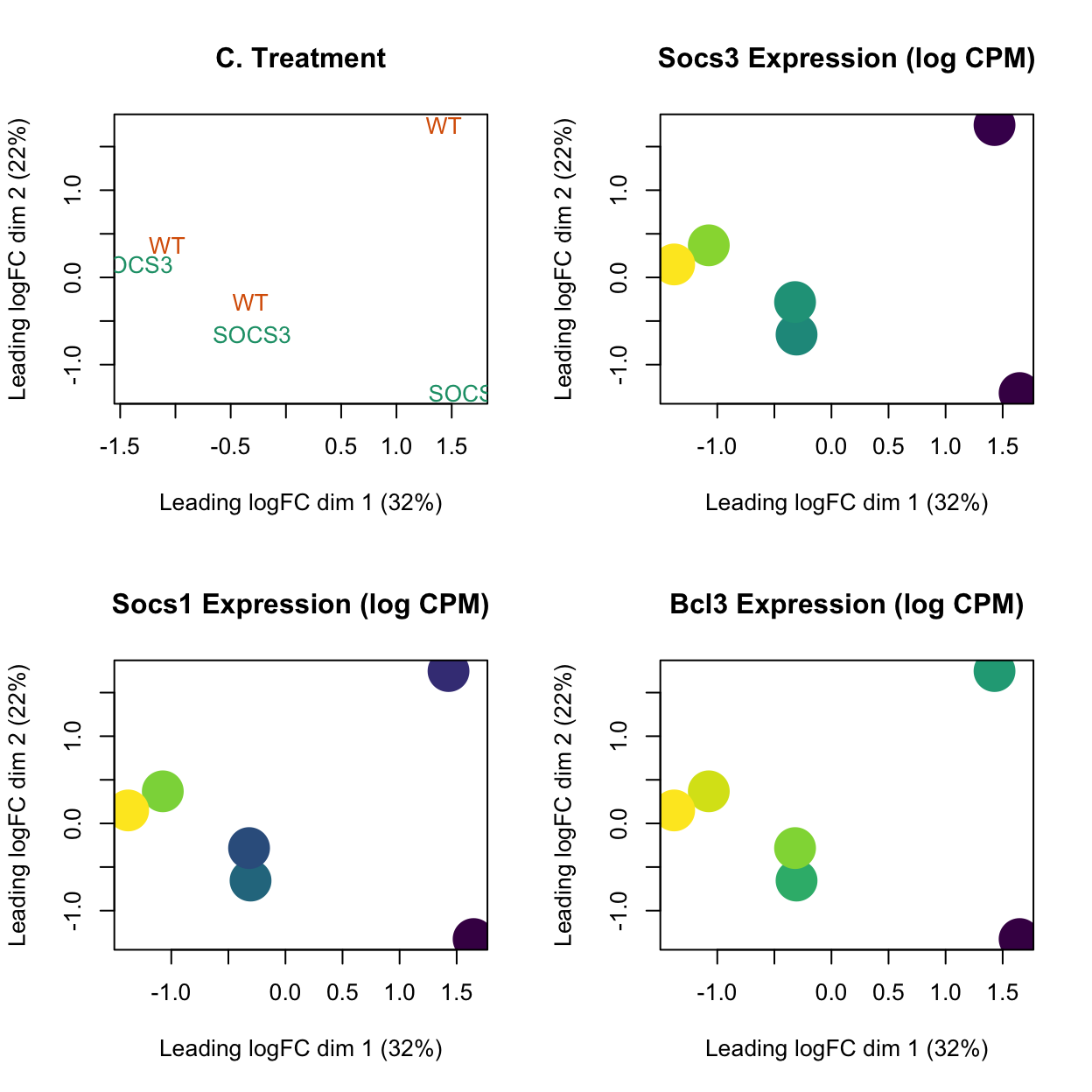

Comparing batches for genes of interest

Based on a priori knowledge, the SOCS3 knockout samples should express Socs1 and Socs3 less than the WT. Bcl3 should be higher in the SOCS3 group.

Show code

genes_of_interest <- c("Socs3", "Socs1", "Bcl3")
selected_genes <- match(genes_of_interest, dge$genes$SYMBOL)

df <- data.frame(
    y = t(lcpm[selected_genes, ]), 
    treatment = dge$samples$treatment, 
    batch = dge$samples$batch)

colnames(df)[1:3] <- genes_of_interest

df$labels <- factor(paste0(df$batch, ".", df$treatment), 
    levels = c("Batch1.WT", "Batch1.SOCS3", "Batch2.WT", "Batch2.SOCS3"))

treatment_colours <- setNames(
    RColorBrewer::brewer.pal(3, "Dark2")[1:2], 
    levels(dge$samples$treatment))

plot_list <- list()
for (i in 1:3) {
    plot_list[[i]] <-
        ggplot(data = df, mapping = aes(x = labels, y = .data[[genes_of_interest[i]]], group = labels, colour = treatment)) + 
            geom_point(size = 4) + 
            theme_minimal() + 
            theme(axis.text.x = element_text(angle = 45, hjust = 1)) + 
            ylab("Expression (log CPM)") + 
            scale_colour_manual(values = treatment_colours) +
            ggtitle(label = paste0(genes_of_interest[i])
    )
}
patchwork::wrap_plots(plot_list, ncol = 3, guides = "collect")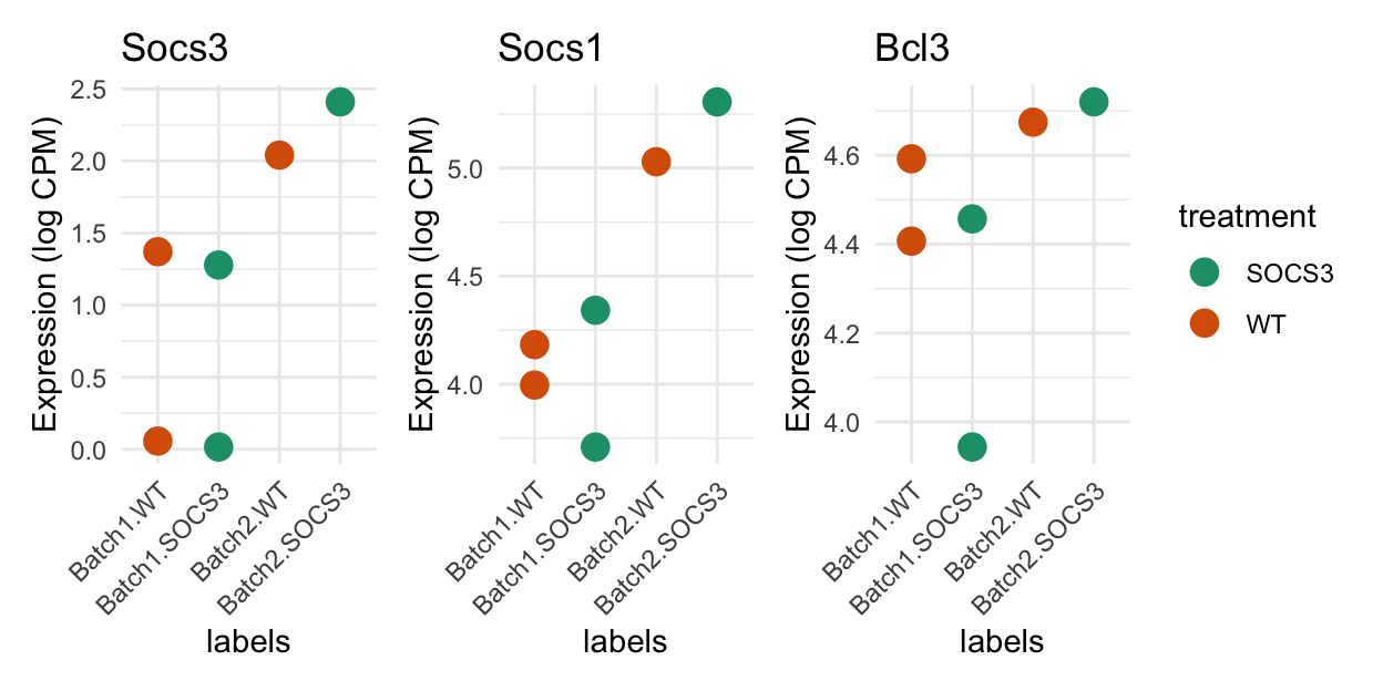

Differential Expression Analyses

Since there is a strong batch effect, we will include batch as a covariate in the differential expression analysis. The analysis below uses the limma::voom() method for differential expression testing.

Show code

design <- model.matrix(~0+treatment+batch, data = dge$samples)

colnames(design) <- gsub("treatment", "", colnames(design))
design

           SOCS3 WT batchBatch2
WT_1_B2        0  1           1
SOCS3_1_B2     1  0           1
SOCS3_2_B1     1  0           0
SOCS3_3_B1     1  0           0
WT_2_B1        0  1           0
WT_3_B1        0  1           0
attr(,"assign")
[1] 1 1 2
attr(,"contrasts")
attr(,"contrasts")$treatment
[1] "contr.treatment"

attr(,"contrasts")$batch
[1] "contr.treatment"

Show code

contr.matrix <- makeContrasts(
   SOCS3vsWT = SOCS3 - WT,
   levels = colnames(design))
contr.matrix

             Contrasts
Levels        SOCS3vsWT
  SOCS3               1
  WT                 -1
  batchBatch2         0

Show code

v <- voom(dge, design, plot=TRUE)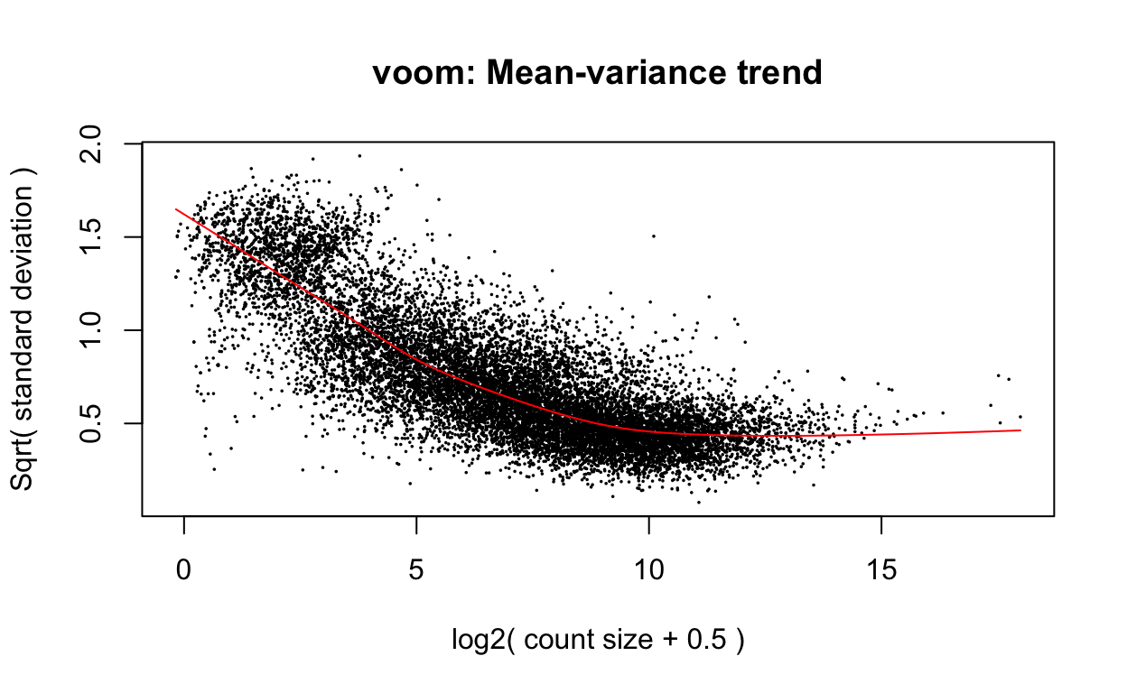

Show code

An object of class "EList"
$genes
             ENSEMBL SYMBOL TXCHROM
1 ENSMUSG00000000001  Gnai3    chr3
3 ENSMUSG00000000028  Cdc45   chr16
4 ENSMUSG00000000037  Scml2    chrX
5 ENSMUSG00000000049   Apoh   chr11
7 ENSMUSG00000000058   Cav2    chr6
13574 more rows ...

$targets
                group lib.size norm.factors  batch treatment
WT_1_B2       WT_1_B2 11948626    1.1514177 Batch2        WT
SOCS3_1_B2 SOCS3_1_B2 13635747    1.1882010 Batch2     SOCS3
SOCS3_2_B1 SOCS3_2_B1 10854339    0.8713582 Batch1     SOCS3
SOCS3_3_B1 SOCS3_3_B1 10697300    0.9910832 Batch1     SOCS3
WT_2_B1       WT_2_B1  9564834    0.9664706 Batch1        WT
WT_3_B1       WT_3_B1  9319320    0.8757532 Batch1        WT
           nFeatures
WT_1_B2        13358
SOCS3_1_B2     13368
SOCS3_2_B1     12831
SOCS3_3_B1     13213
WT_2_B1        13193
WT_3_B1        12746

$E
                    WT_1_B2 SOCS3_1_B2 SOCS3_2_B1 SOCS3_3_B1  WT_2_B1
ENSMUSG00000000001 7.821840   7.810701   8.991167   8.710913 8.808517
ENSMUSG00000000028 5.965225   5.555984   6.390315   6.099478 6.012555
ENSMUSG00000000037 7.383762   7.030364   7.652887   7.273876 7.316380
ENSMUSG00000000049 4.954557   4.646420   2.274045   3.597633 4.121638
ENSMUSG00000000058 5.682147   6.002993   7.270176   7.341961 7.017802
                    WT_3_B1
ENSMUSG00000000001 9.276754
ENSMUSG00000000028 6.503436
ENSMUSG00000000037 7.577031
ENSMUSG00000000049 3.606324
ENSMUSG00000000058 6.877149
13574 more rows ...

$weights
         [,1]     [,2]      [,3]      [,4]      [,5]      [,6]
[1,] 27.30716 27.39838 28.208208 28.194872 28.174692 28.149474
[2,] 19.62372 19.90988 20.906865 20.777044 20.674267 20.439958
[3,] 25.99418 26.20765 26.001644 25.944118 25.795056 25.693540
[4,] 15.05207 11.58310  4.560348  4.509299  6.094405  5.970889
[5,] 18.56868 21.85032 25.724248 25.667488 23.894672 23.743257
13574 more rows ...

$design
           SOCS3 WT batchBatch2
WT_1_B2        0  1           1
SOCS3_1_B2     1  0           1
SOCS3_2_B1     1  0           0
SOCS3_3_B1     1  0           0
WT_2_B1        0  1           0
WT_3_B1        0  1           0
attr(,"assign")
[1] 1 1 2
attr(,"contrasts")
attr(,"contrasts")$treatment
[1] "contr.treatment"

attr(,"contrasts")$batch
[1] "contr.treatment"

Show code

vfit <- lmFit(v, design)
vfit <- contrasts.fit(vfit, contrasts=contr.matrix)

efit <- eBayes(vfit)
plotSA(efit)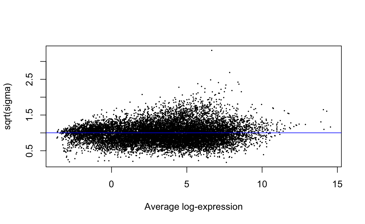

Show code

de_results <- decideTests(efit, adjust.method = "fdr")

The DE results don’t include any significant genes.

Show code

summary(de_results)

       SOCS3vsWT
Down           0
NotSig     13579
Up             0

Show code

topTable(efit, n = 20)

                              ENSEMBL        SYMBOL TXCHROM
ENSMUSG00000028238 ENSMUSG00000028238      Atp6v0d2    chr4
ENSMUSG00000019935 ENSMUSG00000019935       Slc17a8   chr10
ENSMUSG00000030433 ENSMUSG00000030433          Sbk2    chr7
ENSMUSG00000028211 ENSMUSG00000028211     Trp53inp1    chr4
ENSMUSG00000053508 ENSMUSG00000053508         Gtsf2   chr15
ENSMUSG00000025085 ENSMUSG00000025085        Ablim1   chr19
ENSMUSG00000045573 ENSMUSG00000045573          Penk    chr4
ENSMUSG00000072720 ENSMUSG00000072720        Myo18b    chr5
ENSMUSG00000032827 ENSMUSG00000032827       Ppp1r9a    chr6
ENSMUSG00000022150 ENSMUSG00000022150          Dab2   chr15
ENSMUSG00000055632 ENSMUSG00000055632         Hmcn2    chr2
ENSMUSG00000014030 ENSMUSG00000014030          Pax5    chr4
ENSMUSG00000028339 ENSMUSG00000028339       Col15a1    chr4
ENSMUSG00000041870 ENSMUSG00000041870      Ankrd13a    chr5
ENSMUSG00000028163 ENSMUSG00000028163         Nfkb1    chr3
ENSMUSG00000026553 ENSMUSG00000026553          Copa    chr1
ENSMUSG00000043727 ENSMUSG00000043727 F830045P16Rik    chr2
ENSMUSG00000024163 ENSMUSG00000024163      Mapk8ip3   chr17
ENSMUSG00000055360 ENSMUSG00000055360        Prl2c5   chr13
ENSMUSG00000076441 ENSMUSG00000076441          Ass1    chr2
                        logFC  AveExpr         t      P.Value
ENSMUSG00000028238  0.8598567 8.595271  5.399348 0.0002238033
ENSMUSG00000019935  0.5630412 7.988256  3.906128 0.0024923659
ENSMUSG00000030433  1.1506781 5.995617  5.108829 0.0003491585
ENSMUSG00000028211 -0.9642103 9.565562 -3.674647 0.0037144697
ENSMUSG00000053508  0.5985474 6.779710  3.902085 0.0025096690
ENSMUSG00000025085 -0.5157516 7.271214 -3.598688 0.0042390960
ENSMUSG00000045573 -0.5985459 6.322788 -3.875779 0.0026253569
ENSMUSG00000072720  0.5472046 7.110466  3.516553 0.0048929746
ENSMUSG00000032827  0.6508326 6.063368  3.960623 0.0022708415
ENSMUSG00000022150  0.5663092 7.377018  3.238351 0.0079855514
ENSMUSG00000055632  0.7459775 5.731070  4.189640 0.0015415931
ENSMUSG00000014030 -0.9334248 8.378684 -3.128003 0.0097110586
ENSMUSG00000028339  0.6778944 8.366808  3.104799 0.0101196086
ENSMUSG00000041870  0.7214781 6.489920  3.428460 0.0057104239
ENSMUSG00000028163  0.7222143 6.203134  3.659391 0.0038141789
ENSMUSG00000026553 -0.7175525 6.247766 -3.691373 0.0036082358
ENSMUSG00000043727  0.4992752 6.290711  3.301813 0.0071379495
ENSMUSG00000024163  0.7071335 7.192516  3.101426 0.0101804277
ENSMUSG00000055360  0.5931121 6.016363  3.517230 0.0048871826
ENSMUSG00000076441  0.8333460 5.824304  3.680259 0.0036784698
                   adj.P.Val         B
ENSMUSG00000028238 0.9996913 -3.338675
ENSMUSG00000019935 0.9996913 -3.667056
ENSMUSG00000030433 0.9996913 -3.672889
ENSMUSG00000028211 0.9996913 -3.706796
ENSMUSG00000053508 0.9996913 -3.751293
ENSMUSG00000025085 0.9996913 -3.796128
ENSMUSG00000045573 0.9996913 -3.804787
ENSMUSG00000072720 0.9996913 -3.838459
ENSMUSG00000032827 0.9996913 -3.866294
ENSMUSG00000022150 0.9996913 -3.881341
ENSMUSG00000055632 0.9996913 -3.882306
ENSMUSG00000014030 0.9996913 -3.887765
ENSMUSG00000028339 0.9996913 -3.889628
ENSMUSG00000041870 0.9996913 -3.891751
ENSMUSG00000028163 0.9996913 -3.893159
ENSMUSG00000026553 0.9996913 -3.927467
ENSMUSG00000043727 0.9996913 -3.931498
ENSMUSG00000024163 0.9996913 -3.932816
ENSMUSG00000055360 0.9996913 -3.950047
ENSMUSG00000076441 0.9996913 -3.956538

Show code

dir.create(here("output/DEGs/filtered_output_3"), recursive=TRUE)

# Sort the top table by adjusted P value
sorted_de <- topTable(efit, number=Inf, sort.by="P")
sorted_de <- sorted_de[order(sorted_de$adj.P.Val), ]

# Write to a file
write.table(sorted_de, file=here("output/DEGs/filtered_output_3/FO3_DE_results_voom.tsv"),
            sep="\t", quote=FALSE, row.names=FALSE)

A table of the differential expression results are saved in output/DEGs/filtered_output_3/FO3_DE_results_voom.tsv. The rows are sorted so the genes with the lowest adjusted p-value are at the top.

Analysis of Filtered output 3

Introduction

Setting up the data

Reading in count data

Organising sample information

Organising gene annotations

Pre-processing

Filter low quality genes

Quality control

Library size

Number of expressed features

Proportion of mitochondrial genes

Normalisation

Visualising the data

Comparing batches for genes of interest

Differential Expression Analyses